11.3: Energy Carried by Electromagnetic Waves

Learning Objectives

By the end of this section, you will be able to:

• Express the time-averaged energy density of electromagnetic waves in terms of their electric and magnetic field amplitudes
• Calculate the Poynting vector and the energy intensity of electromagnetic waves
• Explain how the energy of an electromagnetic wave depends on its amplitude, whereas the energy of a photon is proportional to its frequency

Anyone who has used a microwave oven knows there is energy in electromagnetic waves. Sometimes this energy is obvious, such as in the warmth of the summer Sun. Other times, it is subtle, such as the unfelt energy of gamma rays, which can destroy living cells.

Electromagnetic waves bring energy into a system by virtue of their electric and magnetic fields. These fields can exert forces and move charges in the system and, thus, do work on them. However, there is energy in an electromagnetic wave itself, whether it is absorbed or not. Once created, the fields carry energy away from a source. If some energy is later absorbed, the field strengths are diminished and anything left travels on.

Clearly, the larger the strength of the electric and magnetic fields, the more work they can do and the greater the energy the electromagnetic wave carries. In electromagnetic waves, the amplitude is the maximum field strength of the electric and magnetic fields (Figure \(\PageIndex{1}\)). The wave energy is determined by the wave amplitude.

Figure \(\PageIndex{1}\): Energy carried by a wave depends on its amplitude. With electromagnetic waves, doubling the E fields and B fields quadruples the energy density u and the energy flux uc.

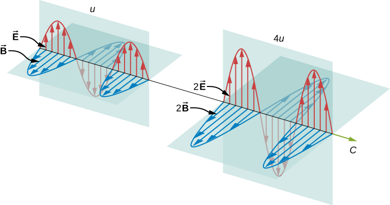
For a plane wave traveling in the direction of the positive x-axis with the phase of the wave chosen so that the wave maximum is at the origin at \(t = 0\), the electric and magnetic fields obey the equations

\[E_y (x,t) = E_0 \, \cos \, (kx - \omega t) \nonumber \]

\[B_x (x,t) = B_0 \, \cos \, (kx - \omega t). \nonumber \]

The energy in any part of the electromagnetic wave is the sum of the energies of the electric and magnetic fields. This energy per unit volume, or energy density u, is the sum of the energy density from the electric field and the energy density from the magnetic field. Expressions for both field energy densities were discussed earlier (\(u_E\) in Capacitance and \(u_B\) in Inductance). Combining these the contributions, we obtain

\[u (x,t) = u_E + u_B = \frac{1}{2}\epsilon_0 E^2 + \frac{1}{2\mu_0} B^2. \nonumber \]

The expression \(E = cB = \frac{1}{\sqrt{\epsilon_0\mu_0}}B\) then shows that the magnetic energy density \(u_B\) and electric energy density \(u_E\) are equal, despite the fact that changing electric fields generally produce only small magnetic fields. The equality of the electric and magnetic energy densities leads to

\[u(x,t) = \epsilon_0 E^2 = \frac{B^2}{\mu_0}. \label{16.27} \]

The energy density moves with the electric and magnetic fields in a similar manner to the waves themselves.

We can find the rate of transport of energy by considering a small time interval \(\Delta t\). As shown in Figure \(\PageIndex{2}\), the energy contained in a cylinder of length \(c\Delta t\) and cross-sectional area A passes through the cross-sectional plane in the interval \(\Delta t\).

Figure \(\PageIndex{2}\): The energy \(uAc\Delta t\) contained in the electric and magnetic fields of the electromagnetic wave in the volume \(Ac\Delta t\) passes through the area \(A\) in time \(\Delta t\).

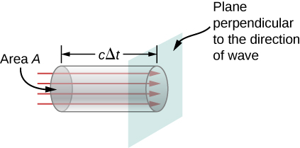
The energy passing through area \(A\) in time \(\Delta t\) is

\[u \times volume = uAc\Delta t. \nonumber \]

The energy per unit area per unit time passing through a plane perpendicular to the wave, called the energy flux and denoted by \(S\), can be calculated by dividing the energy by the area \(A\) and the time interval \(\Delta t\).

\[S = \frac{\text{Energy passing area } A \text{ in time } \Delta t}{A \Delta t} = uc = \epsilon_0cE^2 = \frac{1}{\mu_0} EB. \nonumber \]

More generally, the flux of energy through any surface also depends on the orientation of the surface. To take the direction into account, we introduce a vector \(\vec{S}\), called the Poynting vector, with the following definition:

\[\vec{S} = \frac{1}{\mu_0} \vec{E} \times \vec{B}. \nonumber \]

The cross-product of \(\vec{E}\) and \(\vec{B}\) points in the direction perpendicular to both vectors. To confirm that the direction of \(\vec{S}\) is that of wave propagation, and not its negative, return to Figure 16.3.2. Note that Lenz’s and Faraday’s laws imply that when the magnetic field shown is increasing in time, the electric field is greater at \(x\) than at \(x + \Delta x\). The electric field is decreasing with increasing \(x\) at the given time and location. The proportionality between electric and magnetic fields requires the electric field to increase in time along with the magnetic field. This is possible only if the wave is propagating to the right in the diagram, in which case, the relative orientations show that \(\vec{S} = \frac{1}{\mu_0} \vec{E} \times \vec{B}\) is specifically in the direction of propagation of the electromagnetic wave.

The energy flux at any place also varies in time, as can be seen by substituting \(u\) from Equation 16.3.19 into Equation \ref{16.27}.

\[S(x, t) = c\epsilon_0 E_0^2 \cos^2 \, (kx - \omega t) \label{16.29} \]

Because the frequency of visible light is very high, of the order of \(10^{14} \, Hz\), the energy flux for visible light through any area is an extremely rapidly varying quantity. Most measuring devices, including our eyes, detect only an average over many cycles. The time average of the energy flux is the intensity \(I\) of the electromagnetic wave and is the power per unit area. It can be expressed by averaging the cosine function in Equation \ref{16.29} over one complete cycle, which is the same as time-averaging over many cycles (here, \(T\) is one period):

\[I = S_{avg} = c\epsilon_0E_0^2 \frac{1}{T} \int_0^T \cos^2 \, \left(2\pi \frac{t}{T}\right) dt \label{16.30}. \]

We can either evaluate the integral, or else note that because the sine and cosine differ merely in phase, the average over a complete cycle for \(cos^2 \, (\xi)\) is the same as for \(sin^2 \, (\xi)\), to obtain

\[\langle \cos^2 \xi \rangle = \frac{1}{2} [\langle \cos^2 \xi \rangle + \langle \sin^2 \xi \rangle ] = \frac{1}{2} \langle 1 \rangle = \frac{1}{2}. \nonumber \]

where the angle brackets \(\langle . . . \rangle \) stand for the time-averaging operation. The intensity of light moving at speed \(c\) in vacuum is then found to be

\[I = S_{avg} = \frac{1}{2}c\epsilon_0 E_0^2 \label{16.31} \]

in terms of the maximum electric field strength \(E_0\), which is also the electric field amplitude. Algebraic manipulation produces the relationship

\[I = \frac{cB_0^2}{2\mu_0} \label{16.32} \]

where \(B_0\) is the magnetic field amplitude, which is the same as the maximum magnetic field strength. One more expression for \(I_{avg}\) in terms of both electric and magnetic field strengths is useful. Substituting the fact that \(cB_0 = E_0\), the previous expression becomes

\[I = \frac{E_0B_0}{2\mu_0} \label{16.33}. \]

We can use whichever of the three preceding equations is most convenient, because the three equations are really just different versions of the same result: The energy in a wave is related to amplitude squared. Furthermore, because these equations are based on the assumption that the electromagnetic waves are sinusoidal, the peak intensity is twice the average intensity; that is, \(I_0 = 2I\).

Example \(\PageIndex{1}\): A Laser Beam

The beam from a small laboratory laser typically has an intensity of about \(1.0 \times 10^{-3} W/m^2\). Assuming that the beam is composed of plane waves, calculate the amplitudes of the electric and magnetic fields in the beam.

Strategy

Use the equation expressing intensity in terms of electric field to calculate the electric field from the intensity.

Solution

From Equation \ref{16.31}, the intensity of the laser beam is

\[I = \frac{1}{2}c\epsilon_0 E_0^2. \nonumber \]

The amplitude of the electric field is therefore

\[ \begin{align*} E_0 &= \sqrt{\frac{2}{c\epsilon_0}I} \\[4pt] &= \sqrt{\frac{2}{(3.00 \times 10^8 m/s)(8.85 \times 10^{-12} F/m)}\left(1.0 \times 10^{-3} W/m^2 \right)} \\[4pt] &= 0.87 \, V/m. \end{align*} \]

The amplitude of the magnetic field can be obtained from:

\[B_0 = \frac{E_0}{c} = 2.9 \times 10^{-9} \, T. \nonumber \]

Light Bulb Fields

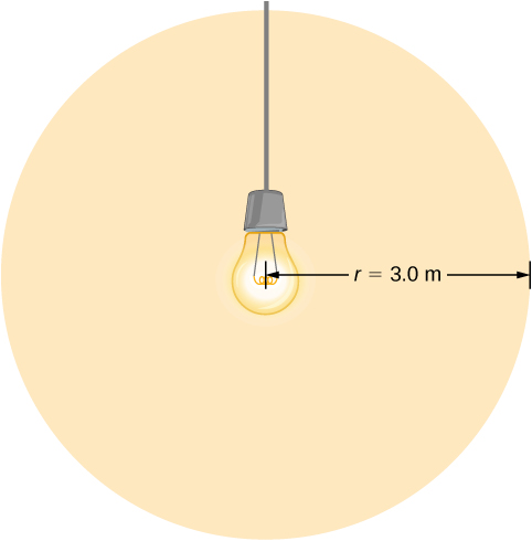
A light bulb emits 5.00 W of power as visible light. What are the average electric and magnetic fields from the light at a distance of 3.0 m?

Strategy

Assume the bulb’s power output P is distributed uniformly over a sphere of radius 3.0 m to calculate the intensity, and from it, the electric field.

Solution

The power radiated as visible light is then

\(I = \frac{P}{4\pi r^2} = \frac{c\epsilon_0 E_0^2}{2},\)

\(E_0 = \sqrt{2\frac{P}{4\pi r^2 c\epsilon_0}} = \sqrt{2\frac{5.00 \, W}{4\pi (3.0 \, m)^2 (3.00 \times 10^8 \, m/s)(8.85 \times 10^{-12} C^2/N \cdot m^2)}} = 5.77 \, N/C,\)

\(B_0 = E_0/c = 1.92 \times 10^{-8} \, T\).

Significance

The intensity I falls off as the distance squared if the radiation is dispersed uniformly in all directions.

Radio Range

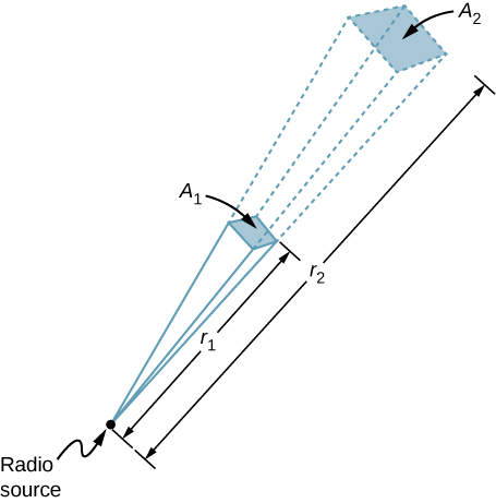
A 60-kW radio transmitter on Earth sends its signal to a satellite 100 km away (Figure \(\PageIndex{3}\)). At what distance in the same direction would the signal have the same maximum field strength if the transmitter’s output power were increased to 90 kW?

Figure \(\PageIndex{3}\): In three dimensions, a signal spreads over a solid angle as it travels outward from its source.

Strategy

The area over which the power in a particular direction is dispersed increases as distance squared, as illustrated in Figure \(\PageIndex{3}\). Change the power output P by a factor of (90 kW/60 kW) and change the area by the same factor to keep \(I = \frac{P}{A} = \frac{c\epsilon_0 E_0^2}{2}\) the same. Then use the proportion of area A in the diagram to distance squared to find the distance that produces the calculated change in area.

Solution

Using the proportionality of the areas to the squares of the distances, and solving, we obtain from the diagram

\[ \begin{align*} \frac{r_2^2}{r_1^2} &= \frac{A_2}{A_1} = \frac{90 \, W}{60 \, W}, \\[4pt] r_2 &= \sqrt{\frac{90}{60}}(100 \, km) \\[4pt] &= 122 \, km. \end{align*} \]

Significance

The range of a radio signal is the maximum distance between the transmitter and receiver that allows for normal operation. In the absence of complications such as reflections from obstacles, the intensity follows an inverse square law, and doubling the range would require multiplying the power by four.