
14.7: Solar Cells


- Last updated
- Aug 27, 2024
- Save as PDF

( \newcommand{\kernel}{\mathrm{null}\,}\)
Now let us look at the opposite process of light generation for a moment. Consider the following situation.
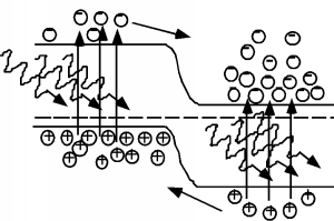 Figure \PageIndex{1}: P-N diode under illumination
We have just a plain old normal p-n junction, only now, instead of applying an external voltage, we imagine that the junction is being illuminated with light whose photon energy is greater than the band-gap. In this situation, instead of recombination, we will get photo-generation of electron hole pairs. The photons simply excite electrons from the full states in the valence band, and "kick" them up into the conduction band, leaving a hole behind. (This is similar to the thermal excitation process we talked about earlier). As you can see from Figure \PageIndex{1}, this creates excess electrons in the conduction band in the p-side of the diode, and excess holes in the valence band of the n-side. These carriers can diffuse over to the junction, where they will be swept across by the built-in electric field in the depletion region. If we were to connect the two sides of the diode together with a wire, a current would flow through that wire as a result of the electrons and holes which move across the junction.
Which way would the current flow? A quick look at Figure \PageIndex{1} shows that holes (positive charge carriers) are generated on the n-side and they float up to the p-side as they go across the junction. Hence positive current must be coming out of the anode, or p-side of the junction. Likewise, electrons generated on the p-side fall down the junction potential, and come out the n-side, but since they have negative charge, this flow represents current going into the cathode. We have constructed a photovoltaic diode, or solar cell! Figure \PageIndex{2} is a picture of what this would look like schematically.
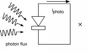 Figure \PageIndex{2}: Schematic representation of a photovoltaic cell
We might like to consider the possibility of using this device as a source of energy, but the way we have things set up now, since the voltage across the diode is zero, and since power equals current times voltage, we see that we are getting nada from the cell. What we need, obviously, is a load resistor, so let's put one in. It should be clear from Figure \PageIndex{3} that the photo current flowing through the load resistor will develop a voltage which it biases the diode in the forward direction, which, of course will cause current to flow back into the anode. This complicates things, it seems we have current coming out of the diode and current going into the diode all at the same time! How are we going to figure out what is going on?
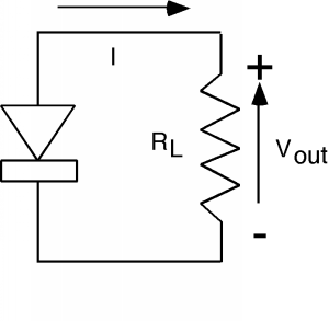 Figure \PageIndex{3}: Photovoltaic cell with a load resistor
The answer is to make a model. The current which arises due to the photon flux can be conveniently represented as a current source. We can leave the diode as a diode, and we have the circuit shown in Figure \PageIndex{4}.
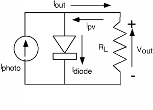 Figure \PageIndex{4}: Model of PV cell
Even though we show I_{\text{out}} coming out of the device, we know by the usual polarity convention that when we define V_{\text{out}} as being positive at the top, then we should show the current for the photovoltaic, I_{\text{pv}}, as going into the diode from the top, which is what was done in Figure \PageIndex{4}. Note that I_{\text{pv}} = I_{\text{diode}} - I_{\text{photo}}, so all we need to do is to subtract the two currents; we do this graphically in Figure \PageIndex{5}. Note that we have numbered the four quadrants in the I \text{-} V plot of the total PV current. In quadrant I and III, the product of I and V is a positive number, meaning that power is being dissipated in the cell. For quadrant II and IV, the product of I and V is negative, and so we are getting power from the device. Clearly we want to operate in quadrant IV. In fact, without the addition of an external battery or current source, the circuit will only run in the IV'th quadrant. Consider adjusting R_{L}, the load resistor from 0 (a short) to \infty (an open). With R_{L} = 0, we would be at point A on Figure \PageIndex{5}. As R_{L} starts to increase from zero, the voltage across both the diode and the resistor will start to increase also, and we will move to point B, say. As R_{L} gets bigger and bigger, we keep moving along the curve until, at point C, where R_{L} is an open and we have the maximum voltage across the device, but, of course, no current coming out!
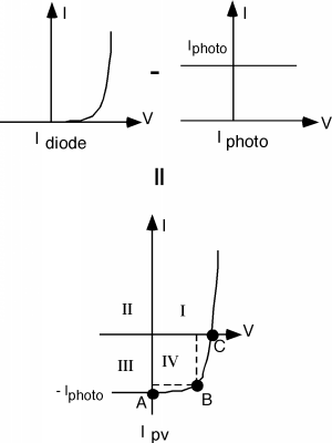 Figure \PageIndex{5}: Combining the diode and the current source
Power is V \cdot I so at B, for instance, the power coming out would be represented by the area enclosed by the two dotted lines and the coordinate axes. Someplace about where I have point B would be where we would be getting the most power our of out solar cell.
Figure \PageIndex{6} shows you what a real solar cell would look like. They are usually made from a complete wafer of silicon, to maximize the usable area. A shallow (0.25 \ \mu \mathrm{m}) junction is made on the top, and top contacts are applied as stripes of metal conductor as shown. An anti-reflection (AR) coating is applied on top of that, which accounts for the bluish color which a typical solar cell has.
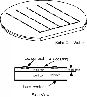 Figure \PageIndex{6}: A real solar cell
The solar power flux on the earth's surface is (conveniently) about 1 \ \frac{\mathrm{kW}}{\mathrm{m}^2}, or 100 \ \frac{\mathrm{mW}}{\mathrm{cm}^2}. So if we made a solar cell from a 4-inch-diameter wafer (typical) it would have an area of about 81 \mathrm{~cm}^2 and so would be receiving a flux of about 8.1 \mathrm{~Watts}. Typical cell efficiencies run from about 10 \ \% to maybe 15 \ \% unless special (and costly) tricks are used. This means that we will get about 1.2 \mathrm{~Watts} out of a single wafer. Looking at point B on Figure \PageIndex{5} we could guess that V_{\text{out}} will be about 0.5 to 0.6 volts, thus we could expect to get maybe around 2.5 amps from a 4-inch wafer at 0.5 volts with 15 \ \% efficiency under the illumination of one sun.