22.7: Equivalent Circuit Model for Reception

In this section, we begin to address antennas as devices that convert incident electromagnetic waves into potentials and currents in a circuit. It is convenient to represent this process in the form of a Thévenin equivalent circuit. The particular circuit addressed in this section is shown in Figure $\PageIndex{1}$.

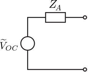Figure $\PageIndex{1}$: Thévenin equivalent circuit for an antenna in the presence of an incident electromagnetic wave. (CC BY-SA 4.0 (modified); S. Lally)

The circuit consists of a voltage source $\widetilde{V}_{OC}$ and a series impedance $Z_A$. The source potential $\widetilde{V}_{OC}$ is the potential at the terminals of the antenna when there is no termination; i.e., when the antenna is open-circuited. The series impedance $Z_A$ is the output impedance of the circuit, and so determines the magnitude and phase of the current at the terminals once a load is connected. Given $\widetilde{V}_{OC}$ and the current through the equivalent circuit, it is possible to determine the power delivered to the load. Thus, this model is quite useful, but only if we are able to determine $\widetilde{V}_{OC}$ and $Z_A$. This section provides an informal derivation of these quantities that is sufficient to productively address the subsequent important topics of effective aperture and impedance matching of receive antennas.¹

Vector effective length

With no derivation required, we can deduce the following about $\widetilde{V}_{OC}$:

• $\widetilde{V}_{OC}$ must depend on the incident electric field intensity $\widetilde{\bf E}^i$. Presumably the relationship is linear, so $\widetilde{V}_{OC}$ is proportional to the magnitude of $\widetilde{\bf E}^i$.
• Since $\widetilde{\bf E}^i$ is a vector whereas $\widetilde{V}_{OC}$ is a scalar, there must be some vector ${\bf l}_e$ for which

  $$\widetilde{V}_{OC}=\widetilde{\bf E}^i\cdot{\bf l}_e \label{m0206_Voc}$$

• Since $\widetilde{\bf E}^i$ has SI base units of V/m and $\widetilde{V}_{OC}$ has SI base units of V, ${\bf l}_e$ must have SI base units of m; i.e., length.
• We expect that $\widetilde{V}_{OC}$ increases as the size of the antenna increases, so the magnitude of ${\bf l}_e$ likely increases with the size of the antenna.
• The direction of ${\bf l}_e$ must be related to the orientation of the incident electric field relative to that of the antenna, since this is clearly important yet we have not already accounted for this.

It may seem at this point that ${\bf l}_e$ is unambiguously determined, and we need merely to derive its value. However, this is not the case. There are in fact multiple unique definitions of ${\bf l}_e$ that will reduce the vector $\widetilde{\bf E}^i$ to the observed scalar $\widetilde{V}_{OC}$ via Equation $\ref{m0206_Voc}$. In this section, we shall employ the most commonly-used definition, in which ${\bf l}_e$ is referred to as vector effective length. Following this definition, the scalar part $l_e$ of ${\bf l}_e=\hat{\bf l} l_e$ is commonly referred to as any of the following: effective length (the term used in this book), effective height, or antenna factor.

In this section, we shall merely define vector effective length, and defer a formal derivation to Section 10.11. In this definition, we arbitrarily set $\hat{\bf l}$, the real-valued unit vector indicating the direction of ${\bf l}_e$, equal to the direction in which the electric field transmitted from this antenna would be polarized in the far field. For example, consider a $\hat{\bf z}$-oriented electrically-short dipole (ESD) located at the origin. The electric field transmitted from this antenna would have only a $\hat{\bf \theta}$ component, and no $\hat{\bf \phi}$ component (and certainly no $\hat{\bf r}$ component). Thus, $\hat{\bf l}=\hat{\bf \theta}$ in this case.

Applying this definition, $\widetilde{\bf E}^i \cdot \hat{\bf l}$ yields the scalar component of $\widetilde{\bf E}^i$ that is co-polarized with electric field radiated by the antenna when transmitting. Now $l_e$ is uniquely defined to be the factor that converts this component into $\widetilde{V}_{OC}$. Summarizing:

The vector effective length ${\bf l}_e = \hat{\bf l} l_e$ is defined as follows: $\hat{\bf l}$ is the real-valued unit vector corresponding to the polarization of the electric field that would be transmitted from the antenna in the far field. Subsequently, the effective length $l_e$ is

$$l_e \triangleq \frac{\widetilde{V}_{OC}}{\widetilde{\bf E}^i \cdot \hat{\bf l}} \nonumber$$

where $\widetilde{V}_{OC}$ is the open-circuit potential induced at the antenna terminals in response to the incident electric field intensity $\widetilde{\bf E}^i$.

While this definition yields an unambiguous value for $l_e$, it is not yet clear what that value is. For most antennas, effective length is quite difficult to determine directly, and one must instead determine effective length indirectly from the transmit characteristics via reciprocity. This approach is relatively easy (although still quite a bit of effort) for thin dipoles, and is presented in Section 10.11.

To provide an example of how effective length works right away, consider the $\hat{\bf z}$-oriented ESD described earlier in this section. Let the length of this ESD be $L$. Let $\widetilde{\bf E}^i$ be a $\hat{\bf \theta}$-polarized plane wave arriving at the ESD. The ESD is open-circuited, so the potential induced in its terminals is $\widetilde{V}_{OC}$. One observes the following:

• When $\widetilde{\bf E}^i$ arrives from anywhere in the $\theta=\pi/2$ plane (i.e., broadside to the ESD), $\widetilde{\bf E}^i$ points in the $-\hat{\bf z}$ direction, and we find that $l_e\approx L/2$. It should not be surprising that $l_e$ is proportional to $L$; this expectation was noted earlier in this section.
• When $\widetilde{\bf E}^i$ arrives from the directions $\theta=0$ or $\theta=\pi$ – i.e., along the axis of the ESD – $\widetilde{\bf E}^i$ is perpendicular to the axis of the ESD. In this case, we find that $l_e$ equals zero.

Taken together, these findings suggest that $l_e$ should contain a factor of $\sin\theta$. We conclude that the vector effective length for a $\hat{\bf z}$-directed ESD of length $L$ is

$${\bf l}_e \approx \hat{\bf \theta}\frac{L}{2}\sin\theta ~~~~~ \mbox{(ESD)} \label{m0206_eVEL-ESD}$$

Example $\PageIndex{1}$: Potential induced in an ESD

A thin straight dipole of length 10 cm is located at the origin and aligned with the $z$-axis. A plane wave is incident on the dipole from the direction $(\theta=\pi/4,\phi=\pi/2)$. The frequency of the wave is 30 MHz. The magnitude of the incident electric field is $10~\mu$V/m (rms). What is the magnitude of the induced open-circuit potential when the electric field is (a) $\hat{\bf \theta}$-polarized and (b) $\hat{\bf \phi}$-polarized?

Solution

The wavelength in this example is $c/f\cong 10$ m, so this dipole is electrically-short. Using Equation $\ref{m0206_eVEL-ESD}$:

$$\begin{aligned} {\bf l}_e & \approx \hat{\bf \theta}\frac{10~\mbox{cm}}{2}\sin\frac{\pi}{4} \nonumber \\ & \approx \hat{\bf \theta}\left(3.54~\mbox{cm}\right) \nonumber\end{aligned} \nonumber$$

Thus, the effective length $l_e=3.54$ cm. When the electric field is $\hat{\bf \theta}$-polarized, the magnitude of the induced open-circuit voltage is

$$\begin{aligned} \left|\widetilde{V}_{OC}\right| &=\left| \widetilde{\bf E}^i \cdot {\bf l}_e \right| \nonumber \\ &\approx \left(10~\mu\mbox{V/m}\right)\hat{\bf \theta} \cdot \hat{\bf \theta}\left(3.54~\mbox{cm}\right) \nonumber \\ &\approx \underline{354~\mbox{nV}~~\mbox{rms}}~~~ \mbox{(a)} \nonumber\end{aligned} \nonumber$$

When the electric field is $\hat{\bf \phi}$-polarized:

$$\begin{aligned} \left|\widetilde{V}_{OC}\right| &\approx \left(10~\mu\mbox{V/m}\right)\hat{\bf \phi} \cdot \hat{\bf \theta}\left(3.54~\mbox{cm}\right) \nonumber \\ &\approx \underline{0} ~~~ \mbox{(b)} \nonumber\end{aligned} \nonumber$$

This is because the polarization of the incident electric field is orthogonal to that of the ESD. In fact, the answer to part (b) is zero for any angle of incidence $(\theta,\phi)$.

Output impedance

The output impedance $Z_A$ is somewhat more difficult to determine without a formal derivation, which is presented in Section 10.12. For the purposes of this section, it suffices to jump directly to the result:

The output impedance $Z_A$ of the equivalent circuit for an antenna in the receive case is equal to the input impedance of the same antenna in the transmit case.

This remarkable fact is a consequence of the reciprocity property of antenna systems, and greatly simplifies the analysis of receive antennas.

Now a demonstration of how the antenna equivalent circuit can be used to determine the power delivered by an antenna to an attached electrical circuit:

Example $\PageIndex{2}$: Power captured by an ESD

Continuing with part (a) of Example $\PageIndex{1}$: If this antenna is terminated into a conjugate-matched load, then what is the power delivered to that load? Assume the antenna is lossless.

Solution

First, we determine the impedance $Z_A$ of the equivalent circuit of the antenna. This is equal to the input impedance of the antenna in transmission. Let $R_A$ and $X_A$ be the real and imaginary parts of this impedance; i.e., $Z_A=R_A+jX_A$. Further, $R_A$ is the sum of the radiation resistance $R_{rad}$ and the loss resistance. The loss resistance is zero because the antenna is lossless. Since this is an ESD:

$$R_{rad} \approx 20\pi^2 \left(\frac{L}{\lambda}\right)^2 \nonumber$$

Therefore, $R_A = R_{rad}\approx 4.93$ m$\Omega$. We do not need to calculate $X_A$, as will become apparent in the next step.

A conjugate-matched load has impedance $Z_A^*$, so the potential $\widetilde{V}_L$ across the load is

$$\widetilde{V}_L = \widetilde{V}_{OC}\frac{Z_A^*}{Z_A+Z_A^*} = \widetilde{V}_{OC}\frac{Z_A^*}{2R_A} \nonumber$$

The current $\widetilde{I}_L$ through the load is

$$\widetilde{I}_L = \frac{\widetilde{V}_{OC}}{Z_A+Z_A^*} = \frac{\widetilde{V}_{OC}}{2R_A} \nonumber$$

Taking $\widetilde{V}_{OC}$ as an RMS quantity, the power $P_L$ delivered to the load is

$$P_L = \mbox{Re}\left\{V_L I_L^*\right\} = \frac{\left|\widetilde{V}_{OC}\right|^2}{4R_A} \nonumber$$

In part (a) of Example $\PageIndex{1}$, $\left|\widetilde{V}_{OC}\right|$ is found to be $\approx 354$ nV rms, so $P_L \approx \underline{6.33 \text{ pW}}$.

---

1. Formal derivations of these quantities are provided in subsequent sections. The starting point is the section on reciprocity.↩