
23.3: Radio Signal Metrics


- Last updated
- Aug 27, 2024
- Save as PDF

( \newcommand{\kernel}{\mathrm{null}\,}\)
Radio signals are engineered to trade-off efficient use of the EM spectrum with the complexity and performance of the required RF hardware. Ultimately the goal is to efficiently use spectrum through maximal packing of information, e.g. digital bits, in a given bandwidth while, for mobile radios especially, using as little prime power as possible. The choice of the type of modulation to use is at the core of the communication system design tradeoff.
There are two families of modulation methods: analog and digital modulation. In analog modulation the RF signal has a continuous range of values; in digital modulation, the output has a number of discrete states at particular times called clock ticks, say every microsecond. There are just a few modulation schemes, all of which are digital, that achieve the optimum trade-offs of spectral efficiency and ease of use with acceptable hardware complexity. If hardware complexity is not a concern, which modulation scheme is used depends on noise and interference as well as the power required to transmit a signal, and the power required to process a received signal.
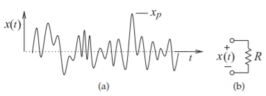
Figure 23.3.1: Definition of crest factor: (a) arbitrary waveform; and (b) voltage across a resistor.
This section introduces several metrics that characterize the variability of the amplitude of a modulated signal, and this variability has a direct impact on how analog hardware performs are designed and how efficiently hardware can be used.
2.2.1 Crest Factor and Peak-to-Average Power Ratio
Introduction
In radio engineering crest factor (CF) is a metric that describes how the voltage of a modulated carrier signal varies with time, and peak-to-average power ratio (PAPR) describes how the instantaneous power of a carrier signal varies with time. Be aware that there is one metric, peak-to-average ratio (PAR), that is defined differently in the power, communications theory, and microwave communities. In some communities CF is also called the peak-to-average ratio (PAR). This can leads to problems. Consider, for example, the community that works on smart power metering which combines power measurement, communications theory, and microwave design. The solution to this inevitable confusion is to skip the use of PAR and use unambiguous metrics.
Note
In standards PAR is defined as the ratio of the instantaneous peak value of a signal parameter to its time-averaged value. PAR is used with many signal parameters, e.g. voltage, current, power, and frequency [1].
Crest Factor
CF is the ratio of the maximum signal, such as a voltage, to its root-meansquare (rms) value. Referring to the arbitrary waveform shown in Figure 23.3.1(a), xp is the absolute peak value of the waveform x(t), if xrms is its rms value, then the crest factor is [2]
CF=xp/xrems
More formally,
CF=‖x‖∞‖x‖2
where ‖x‖∞ is the infinity norm, and here is the maximum value of x(t), ‖x‖∞=max[x(t)]=xp, and ‖x‖2 is just the rms value of x(t):
xrms=‖x‖2=limT→∞√1T∫T0x(t)⋅dt
Note that CF is a voltage (or current) ratio rather than a power ratio. The CFs of several waveforms are given in Table 23.3.1.
Peak-to-Average Power Ratio (PAPR)
The peak-to-average power ratio (PAPR) is analogous to CF but for power. If x(t) is the voltage across a resistor, as shown in Figure 23.3.1(b), then the
| Waveform | x(t) | Max. value | rms (xrms) | CF | PAPR |
|---|---|---|---|---|---|
| DC | 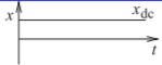 |
xdc | xdc | 1 | 0 dB |
| Sinewave | 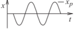 |
xp | xp√2 | 1.414 | 3.01 dB |
| Full-wave rectified sinewave | 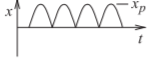 |
xp | xp√2=0.717xp | 1.414 | 3.01 dB |
| Half-wave rectified sinewave | 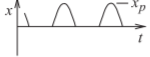 |
xp | xp2 | 2 | 6.02 dB |
| Triangle wave | 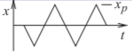 |
xp | xp√3=0.577xp | 1.732 | 4.77 dB |
| Square wave | 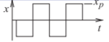 |
xp | xp | 1 | 0 dB |
Table 23.3.1
instantaneous peak power in the resistor is
Pp=|xp|2/R
where again xp is the peak absolute value of the waveform. Pp is the power of the peak of a waveform treating it as though it was a DC signal. This is appropriate for a slowly varying signal such as a power frequency signal as it is this instantaneous power that determines thermal disruption of a power system. It is not the appropriate power to use with radio signals and a more suitable microwave signal metric is described in Section 2.2.2. The average power dissipated in the resistor is
Pavg=|xrms|2/R
Then
PAPR=PpPavg=CF2=(xp/xrms)2
In decibels,
PAPR|dB=10log(PAPR)=20log(CF)=20log(xp/xrms)
The definition of PAPR above can be used with any waveform and can be used in all branches of electrical engineering. The PAPRs of several waveforms are given in Table 23.3.1.
Example 23.3.1: Crest Factor and PAPR of an Offset Sinusoid
What is the crest factor (CF) and peak-to-average power ratio (PAPR) of the signal x(t)=0.1+0.5sin(ωt)?
Solution
The signal is a sinusoid offset by a DC term. The peak value of x(t) is xp=0.6, and the rms value of the signal will be the square root of the rms values squared of the individual DC and sinusoidal components. This applies to any composite signal provided that the components are uncorrelated. So xrms=√0.12+(0.5/√2)2=0.3674. The general solution for a signal x(t)=a+bsin(ωt) is, using Equation (???),
xrms=√limT→∞1T∫T0[x(t)]2dt=√limT→∞1T∫T0[a+bsin(ωt)]2dt=√limT→∞1T∫T0[a2+absin(ωt)+b2sin2(ωt)]dt=√limT→∞1T{∫T0a2dt+∫T0absin(ωt)dt+∫T0b212[1+cos(2ωt)]dt}=√limT→∞1T{a2Tdt+0+12b2T}
since the integral of sin and cos over a period is zero. Thus
xrms=√a2+b2/2=√0.12+120.52=0.3674
the crest factor is
CF=xpxrms=0.60.3674=1.6311
and PAPR is
PAPR=20log(1.6311)=4.260 dB
There is a quicker way of calculating PAPR by dealing with the powers directly. The peak power of the waveform is Pp=x2p/R=0.62/R=0.36/R, where x is being treated as a voltage across a resistor R. The two parts of x(t), i.e. the DC component and the sinewave, are uncorrelated, so the average power of the combined signal is the sum of the powers of the uncorrelated components, so
Pavg=1R[0.12+120.52]1R=0.1350R
Thus, in decibels,
PAPR|dB=10log(PpPavg)=x2px2rms=10log(0.360.135)=10log(2.667)=4.260 dB
2.2.2 Peak-to-Mean Envelope Power Ratio
Another metric for characterizing signals is the peak-to-mean envelope power ratio (PMEPR) and this is particularly useful for modulated signals. The amount of information sent by a communication signal is proportional to its average power, however, RF hardware must be designed with enough margin to be able to handle peaks in the signal without producing appreciable distortion. The waveform of a narrowband modulated signal appears as a carrier that slowly changes in amplitude and phase. One sinewave of this modulated signal is called a pseudo-carrier and the power of one cycle of the pseudo-carrier when the amplitude of the modulated signal is at its maximum (i.e. at the peak of the envelope) is called the peak envelope power (PEP) [1] (PEP=PPEP). The ratio of PEP to the average signal power (the power averaged over all time) is called the PMEPR.
Then if the average power of the modulated signal is Pavg
PMEPR=PEPPavg=PPEPPavg
PMEPR is a good indicator of how sensitive a modulation format is to distortion introduced by the nonlinearity of RF hardware [3].
It is complex to determine the PMEPR for a general modulated signal. Below the mathematics is presented for an AM signal with a sinusoidal modulating signal. Determining the PMEPR otherwise requires numerical integration following the procedure outlined below.
PMEPR of an AM Signal
A good estimate of the PMEPR of an AM signal can be obtained by considering a sinusoidal modulating signal (rather than an actual baseband signal). Let y(t)=cos(2πfmt) be a cosinusoidal modulating signal with frequency fm. Then, for AM, the modulated carrier signal is
x(t)=Ac[1+mcos(2πfmt)]cos(2πfct)
where m is the modulation index (e.g. 100% AM has m=1). Thus if the power of just one quasi-period of x(t), i.e. one cycle of the pseudo carrier, is considered then x(t) has a power that varies with time.
Consider a voltage v(t) across a resistor of conductance G. The power of the signal is determined by integrating over all time, which is work, and dividing by the time period. This yields the average power:
Pavg=limτ→∞∫τ−τ12τGv2(t)dt
Now, if v(t) is a sinusoidal, v(t)=Acosωt, then
Pavg=limτ→∞12τ∫τ−τA2cGcos2(ωt)dt=limτ→∞12τ∫τ−τA2cG12[1+cos(2ωt)]dt=12A2cG{limτ→∞12τ∫τ−τ1dt+limτ→∞12τ∫τ−τcos(2ωt)dt}=12A2cG
In the above equation, a useful equivalence has been employed by observing that the infinite integral of a cosinusoid can be simplified to just integrating over one period, T=2π/ω:
limτ→∞12τ∫τ−τcosn(ωt)dt=1T∫T/2−T/2cosn(ωt)dt
where n is a positive integer. In power calculations there are a number of other useful simplifying techniques based on trigonometric identities. Some of the ones that will be used here are the following:
cosAcosB=12[cos(A−B)+cos(A+B)]cos2A=12[1+cos(2A)]limτ→∞12τ∫τ−τcosωtdt=1T∫T/2−T/2cos(ωt)dt=01T∫T/2−T/2cos2(ωt)dt=1T∫T/2−T/212[cos(2ωt)+cos(0)]=12T[∫T/2−T/2cos(2ωt)dt+∫T/2−T/21dt]=12T(0+T)=12
More trigonometric identities are given in Appendix 1.A.2 of [4]. Also, when cosinusoids cosωAt and cosωBt, having different frequencies (ωA≠ωB), are multiplied together, for large τ,
∫τ−τcosωAtcosωBtdt=∫τ−τ12[cos(ωA+ωB)t+cos(ωA−ωB)t]dt=0
and if ωA≠ωB≠0
∫∞−∞cosωAtcosnωBtdt=0
Now the discussion returns to characterizing an AM signal by considering the long-term average power and the maximum short-term power of the signal. The pseudo-carrier at its peak amplitude is, from Equation (???),
xp(t)=Ac[1+m]cos(2πfct)
Then the power (PPEP) of the peak pseudo carrier is obtained by integrating over one period of the pseudo carrier:
PPEP=1T∫T/2−T/2Gx2(t)dt=1T∫T/2−T/2A2cG(1+m)2cos2(ωct)dt=A2cG(1+m)21T∫T/2−T/2cos2(ωct)dt=12A2cG(1+m)2
The average power (Pavg) of the modulated signal is obtained by integrating over all time, so
Pavg=limτ→∞12τ∫τ−τGx2(t)dt=A2cGlimτ→∞12τ∫τ−τ{[1+mcos(ωmt)]cos(ωct}2dt=A2cGlimτ→∞12τ∫τ−τ{[1+2mcos(ωmt)+m2cos2(ωmt)]cos2(ωct)}dt=A2cG[limτ→∞12τ∫τ−τcos2(ωct)dt+limτ→∞12τ∫τ−τ2mcos(ωmt)cos2(ωct)dt+limτ→∞12τ∫τ−τm2cos2(ωmt)cos2(ωct)dt]=A2cG{12+0+m2limτ→∞12τ∫τ−τ14[1+cos(2ωmt)][1+cos(2ωct)]dt}=A2cG{12+m24[limτ→∞12τ∫τ−τ1dt+limτ→∞12τ∫τ−τcos(2ωmt)dt+limτ→∞12τ∫τ−τcos(2ωct)dt+limτ→∞12τ∫τ−τcos(2ωmt)cos(2ωct)dt]}=A2cG[12+m2(14+0+0+0)]=12A2cG(1+m2/2)
Thus the rms voltage, xrms, can be determined as Pavg=x2rmsG. So the PMEPR of an AM signal (i.e., PMEPRAM) is
PMEPRAM=PPEPPavg=12A2cG(1+m)212A2cG(1+m2/2)=(1+m)21+m2/2
For 100% AM described by m=1, the PMEPR is
PMEPR100%AM=(1+1)21+12/2=41.5=2.667=4.26 dB
In expressing the PMEPR in decibels, the formula PMEPRdB=10log(PMEPR) is used as PMEPR is a power ratio. As an example, for 50% AM, described by m=0.5, the PMEPR is
PMEPR50%AM=(1+0.5)21+0.52/2=2.251.125=2=3 dB
2.2.3 Two-Tone Signal
In assessing, either through laboratory measurements or simulations, it is common and often necessary to use very simple representations of a baseband signal or even of a modulated signal. This greatly simplifies matters and there is a justified expectation that the performance with the test signal is a good indication of performance with an actual baseband or modulated signal. With simulation at the circuit level it is usually impossible to consider real baseband signals as simulation may not even be possible or simulation may take unacceptable times. Instead it is common to use single-tone, i.e. single sinewave, or two-tone signals. A two-tone signal is a signal that is the sum of two cosinusoids:
y(t)=XAcos(ωAt)+XBcos(ωBt)
Generally the frequencies of the two tones are close (|ωA−ωB|≪ωA), with the concept being that both tones fit within the passband of a transmitter’s or receiver’s bandpass filters. A two-tone signal is not a form of modulation, but is commonly used to characterize the nonlinear performance of RF systems and has an envelope that is similar to that of many modulated signals. The composite signal, y(t), looks like a pseudo-carrier with a slowly varying amplitude, not unlike an AM signal. The tones are uncorrelated so that the average power of the composite signal, y(t), is the sum of the powers of each of the individual tones. The peak power of the composite signal is that of the peak pseudo-carrier, so y(t) has a peak amplitude of XA+XB. The peak pseudo carrier is the single RF sinusoid where the sinusoid of each sinusoid align as much as possible. Similar concepts apply to three-tone and n-tone signals.
Example 23.3.2: PMEPR of a Two-Tone Signal
What is the PMEPR of a two-tone signal with the tones having equal amplitude?
Solution
Let the amplitudes of the two tones be XA and XB. Now XA=XB=X, and so the peak pseudo-carrier has amplitude 2X, and the power of the peak RF carrier is proportional to 12(2X)2=2X2. The average power is proportional to 12(X2A+X2B)=12(X2+X+2)=X2, as each tone is independent of the other and so the powers can be added.
PMEPR=PPEPPavg=2X2X2=2=3 dB
Example 23.3.3: PMEPR of Uncorrelated Signals
Consider the combination of two uncorrelated analog signals, e.g. a two-tone signal. One signal is denoted x(t) and the other y(t), where x(t)=0.1sin(109t) and y(t)=0.05sin(1.01·109t). What is the PMEPR of this combined signal?
Solution
These two signals are uncorrelated and this is key in determining the average power, Pavg, as the sum of the powers of each individual signal (k is a proportionality constant):
Pavg=∫∞−∞x2(t)⋅dt+∫∞−∞y2(t)⋅dt=k2(0.1)2+k2(0.5)2=k2[0.01+0.0025]=0.00625k
The two carriers are close in frequency so that the sum signal z(t)=x(t)+y(t) looks like a slowly varying signal with a radian frequency near 109 rads per second. The peak amplitude of one pseudo-cycle of z(t)is0.1+0.05=0.15. Thus the power of the largest cycle is
PPEP=12k(0.15)2=0.01125k
and so
PMEPR=PPEPPavg=0.011250.00625=1.8=2.55 dB
Summary
The PMEPR is an important attribute of a modulation format and impacts the types of circuit designs that can be used. It is much more challenging to develop power-efficient hardware introducing only low levels of distortion when the PMEPR is high.
It is tempting to consider if the lengthy integrations can be circumvented. Powers can be added if the signal components (the tones making up the signal) are uncorrelated. If they are correlated, then the complete integrations are required. Consider two uncorrelated sinusoids of (average) powers P1 and P2, respectively, then the average power of the composite signal is Pavg=P1+P2. However, in determining the peak sinusoidal power, the RF cycle where the two largest pseudo-carrier sinusoids align is considered, and here the voltages add to produce a single cycle of a sinewave with a higher amplitude. So peak power applies to just one RF pseudo-cycle. Generally the voltage amplitude of the two sinewaves would be added and then the power calculated. If the uncorrelated carriers are modulated and the modulating signals (the baseband signals) are uncorrelated, then the average power can be determined in the same way, but the peak power calculation is much more complicated. The integrations are the only calculations that can always be relied on and can be used with all modulated signals.
Note
Signals x(t) and y(t) are uncorrelated if the integral over all time and time offsets of their product is zero: C=∫+∞−∞x(t)y(t+τ)dt=0 for all τ.
The preferred usage of PAR, PAPR, or PMEPR in RF and microwave engineering is currently in a transition phase. The most common usage of PAR and PAPR in electrical engineering refers to the peak of a signal as being the instantaneous peak value, and in the case of PAPR, the instantaneous power of the signal is calculated as if the peak is a DC value. In the past, many RF and microwave publications have taken the peak as the peak power of a sinusoid having an amplitude equal to the peak voltage of the signal and used that to calculate PAR. This usage is inconsistent with the predominant usage in electrical engineering and is a particular problem when using wireless technology in other disciplines. PMEPR is the preferred usage for what RF and microwave engineers intend to refer to when using the term PAR. A reader of RF literature encountering PAR needs to determine how the term is being used. There is no confusion if PMEPR is used.
Example 23.3.4: PAPR and PMEPR of an AM Signal
What is the PAPR and PMEPR of a 100% AM signal?
Solution
The signal is x(t)=Ac[1+cos2πfmt]cos2πfct and the PMEPR of this signal, from Equation (???), is 4.26 dB. Now PAPR uses the absolute maximum value of the signal rather than the maximum short-term power of the envelope. The peak value of x(t) is 2Ac so the peak power (if the signal is a voltage across a conductance G) is
Ppeak, PAPR=(2Ac)2G
Pavg is the same for PAPR and PMEPR for the AM signal, see Equation (23.3.33), so that
PAPR=Ppeak, PAPRPavg=(2Ac)2G12A2c(1+12)=43/4=163=5.333=7.27 dB
So PAPR is 3 dB higher than PMEPR for a 100% modulated AM signal, see Equation (???). This is not always the case for other modulation schemes.