
9.5: Examples


- Last updated
- Oct 2, 2023
- Save as PDF

( \newcommand{\kernel}{\mathrm{null}\,}\)
I have a spring with a spring constant 1750 N/m and a mass 13.5 kg attached to the end. They are oriented horizontally so the mass is sliding across a frictionless surface.
- I pull the spring a distance 5.4 cm from equilibrium. How much energy did I add on the system?
- I let the mass go; what velocity is it traveling with when it crosses the equilibrium point?
- The mass travels through the equilibrium point and stops at the maximum compression point of the spring. How far is the mass from the equilibrium point?
- How much energy did the mass transfer to the spring as it moved from equilibrium to the maximum compression point?
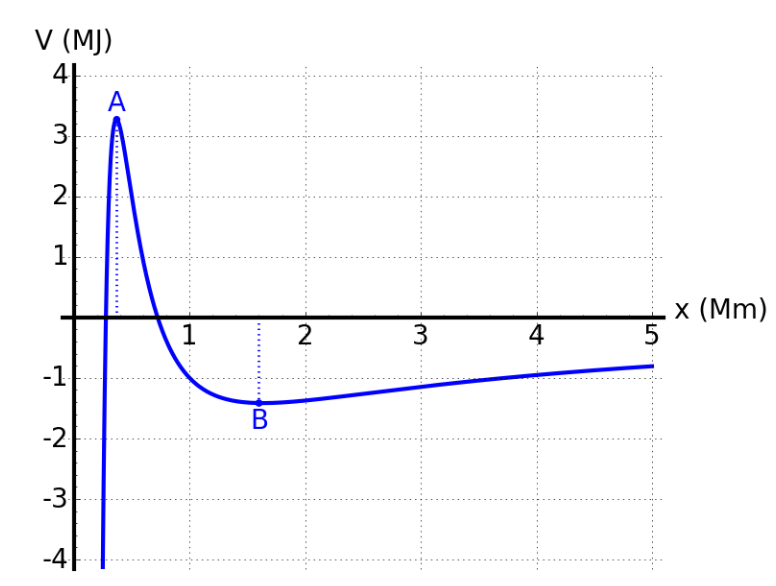
The figure above shows the gravitational potential energy interaction between two massive planets orbiting around each other. At x = ∞, this potential is zero.
- Indicate the sign of the force associated to this potential for each of the three regions in the following table.
Between 0 and A Between A and B Between B and ∞ F positive or Negative? - If the two planets are initially separated by a large distance, but are moving towards each other with a kinetic energy of 1.0 MJ, about how close will they get to each
other?
You are designing a back-up safety system for an elevator, that will catch the elevator on a spring if the cable breaks. The mass of the elevator is 750 kg, and the system needs to be able to stop an elevator that dropped a distance 10 m before hitting the spring, but only compressing a distance 2 m.
What does the spring constant have to be for this safety system to work as designed?
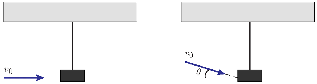
A ballistic pendulum can be used to determine the muzzle speed of a gun. The bullet is fired into a hanging pendulum, and by measuring how far into the air the pendulum swings you can figure out how fast the bullet was traveling.
- First determine the mass of the pendulum: I fire a bullet of mass 70 g straight into the pendulum block (left figure), at a speed of 500 m/s, and I measure that the block rises 62 cm into the air.
- Now I take another gun which fires the same size bullet, and find the pendulum rises a height of 75 cm. How fast did the second gun fire the bullet?
- What if I wasn't very careful when I aimed the bullet? If I fired at a 7.5∘ angle with respect to the horizontal (right figure), what was the true muzzle speed of the gun?
The potential energy for a particle undergoing one-dimensional motion along the x-axis is U(x) = 2(x4 − x2), where U is in joules and x is in meters. The particle is not subject to any non-conservative forces and its mechanical energy is constant at E = −0.25 J. (a) Is the motion of the particle confined to any regions on the x-axis, and if so, what are they? (b) Are there any equilibrium points, and if so, where are they and are they stable or unstable?
Strategy
First, we need to graph the potential energy as a function of x. The function is zero at the origin, becomes negative as x increases in the positive or negative directions (x2 is larger than x4 for x < 1), and then becomes positive at sufficiently large |x|. Your graph should look like a double potential well, with the zeros determined by solving the equation U(x) = 0, and the extremes determined by examining the first and second derivatives of U(x), as shown in Figure 9.5.3.
You can find the values of (a) the allowed regions along the x-axis, for the given value of the mechanical energy, from the condition that the kinetic energy can’t be negative, and (b) the equilibrium points and their stability from the properties of the force (stable for a relative minimum and unstable for a relative maximum of potential energy). You can just eyeball the graph to reach qualitative answers to the questions in this example. That, after all, is the value of potential energy diagrams.
You can see that there are two allowed regions for the motion (E > U) and three equilibrium points (slope dUdx = 0), of which the central one is unstable (d2Udx2<0), and the other two are stable (d2Udx2>0).
Solution
- To find the allowed regions for x, we use the condition K=E−U=−14−2(x4−x2)≥0. If we complete the square in x 2 , this condition simplifies to 2(x2−12)2≤14, which we can solve to obtain 12−√18≤x2≤12+√18.This represents two allowed regions, xp ≤ x ≤ xR and −xR ≤ x ≤ − xp, where xp = 0.38 and xR = 0.92 (in meters).
- To find the equilibrium points, we solve the equation dUdx=8x3−4x=0and find x = 0 and x = ±xQ, where xQ = 1√2 = 0.707 (meters). The second derivative d2Udx2=24x2−4is negative at x = 0, so that position is a relative maximum and the equilibrium there is unstable. The second derivative is positive at x = ±xQ, so these positions are relative minima and represent stable equilibria.
Significance
The particle in this example can oscillate in the allowed region about either of the two stable equilibrium points we found, but it does not have enough energy to escape from whichever potential well it happens to initially be in. The conservation of mechanical energy and the relations between kinetic energy and speed, and potential energy and force, enable you to deduce much information about the qualitative behavior of the motion of a particle, as well as some quantitative information, from a graph of its potential energy.
Repeat Example 9.5.1 when the particle’s mechanical energy is +0.25 J.
A block of mass m is sliding on a frictionless, horizontal surface, with a velocity vi. It hits an ideal spring, of spring constant k, which is attached to the wall. The spring compresses until the block momentarily stops, and then starts expanding again, so the block ultimately bounces off.
- In the absence of dissipation, what is the block’s final speed?
- By how much is the spring compressed?
Solution
This is a simpler version of the problem considered in Section 5.1, and in the next example. The problem involves the conversion of kinetic energy into elastic potential energy, and back. In the absence of dissipation, Equation (5.4.1), specialized to this system (the spring and the block) reads:
K+Uspr= constant
For part (a), we consider the whole process where the spring starts relaxed and ends relaxed, so Uspri=Usprf = 0. Therefore, we must also have Kf=Ki, which means the block’s final speed is the same as its initial speed. As explained in the chapter, this is characteristic of a conservative interaction.
For part (b), we take the final state to be the instant where the spring is maximally compressed and the block is momentarily at rest, so all the energy in the system is spring (which is to say, elastic) potential energy. If the spring is compressed a distance d (that is, x−x0=−d in Equation (5.1.5)), this potential energy is 12kd2, so setting that equal to the system’s initial energy we get:
Ki+0=0+12kd2
or
12mv2i=12kd2
which can be solved to get
d=√mkvi.