8.9: Geometric Interpretations

Recall these ideas from your study of the calculus:

• The derivative of a function \(f(t)\) with respect to \(t\) at any time \(t\) is the slope of the tangent to the curve at \(t\).
• The integral of a function \(f(t)\) with respect to \(t\) is the area under the curve (with negative \(f\) counting as negative area).

Now if you're given a formula for \(x(t)\), you can use \(v=d x / d t\) to find a formula for the velocity \(v\). But suppose that instead of a formula, you're given a data table or plot of \(x\) vs. \(t .{ }^{4}\) Then you can find the velocity at any time by finding the slope of the curve at that point—which is geometrically the same thing as finding the derivative.

Similarly, if you're given a formula for \(v(t)\), you can use \(x=\int v d t\) to find a formula for the position \(x\). Suppose, though, that instead of a formula, you have a data table or plot of \(v\) vs. \(t\). Then you can find the net distance traveled between times \(t_{1}\) and \(t_{2}\) by finding the area under the \(v\) vs. \(t\) curve between times \(t_{1}\) and \(t_{2}\).

For example, consider the motion of a particles that moves in one dimension according to \(x(t)=5 t^{2}+\) \(3 t+7\) (where \(x\) is in meters and \(t\) is in seconds), as illustrated in Figure \(\PageIndex{1}\). The position \(x\) at any time \(t\) is shown by the parabolic curve in Figure \(\PageIndex{1}\)(a); you can read off the position of the particle at any time just by looking at the graph. The slope of the graph at any time gives the velocity at that time. For example, at \(t=30 \mathrm{sec}\), we can draw a straight line tangent to the curve, as shown in Fig. \(\PageIndex{1}\)(a); measuring the slope of that line (as the "rise" divided by the "run"), we find \(v(30 \mathrm{sec})=33 \mathrm{~m} / \mathrm{s}\).

Figure \(\PageIndex{1}\): Plots of position, velocity, and acceleration vs. time for a particle moving according to \(x(t)=\) \(5 t^{2}+3 t+7 \mathrm{~m}\). From the calculus, we find (b) \(v(t)=d x / d t=10 t+3 \mathrm{~m} / \mathrm{s}\), and (c) \(a(t)=d v / d t=10\) \(\mathrm{m} / \mathrm{s}^{2}\). The same results are found geometrically, as described in the text.

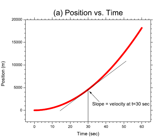
Figure \(\PageIndex{1}\)(b) shows velocity vs. time for the same particle. In this case, you can read off the velocity \(v\) at any time \(t\) by inspection of the plot. The slope of the plot at any time \(t\) gives the acceleration at that time. In this case, the plot of \(v\) vs. \(t\) is a straight line with constant slope, so the acceleration is the same at all times: \(a=10 \mathrm{~m} / \mathrm{s}^{2}\). The area under the curve gives the change in position between two times. For example, again in Fig. \(\PageIndex{1}\)(b), the area under the \(v\) vs. \(t\) curve from \(t=20 \mathrm{sec}\) to \(t=50 \mathrm{sec}\) (the area of a trapezoid in this case) gives the change in position during that time interval: \(10,590 \mathrm{~m}\).

Figure \(\PageIndex{1}\)(c) shows acceleration vs. time for the same particle. As before, you can read off the acceleration \(a\) at any time \(t\) by inspection of the plot. In this case, the acceleration is a constant \(10 \mathrm{~m} / \mathrm{s}^{2}\) for all times. The slope of the plot at any time \(t\) gives the jerk at that time. In this case, since the line is horizontal with zero slope, the jerk is zero at all times. The area under the curve in Fig. 5.1(c) gives the change in velocity between two times. For example, the area under the curve between \(t=20 \mathrm{sec}\) and \(t=50 \mathrm{sec}\) gives the velocity change during that interval, \(300 \mathrm{~m} / \mathrm{s}\). This may be confirmed in Fig. \(\PageIndex{1}\)(b): the velocity changes from \(203 \mathrm{~m} / \mathrm{s}\) at \(t=20 \mathrm{sec}\) to \(503 \mathrm{~m} / \mathrm{s}\) at \(t=50 \mathrm{sec}\).

---

4. The word versus (vs.) has a specific meaning in plots: it's always the ordinate vs. the abscissa (e.g. \(y\) vs. \(x\) ).