2.4: Problem-Solving for Basic Kinematics
- Last updated
- Jan 14, 2019
- Save as PDF
- Page ID
- 16931

- Boundless
- Boundless
( \newcommand{\kernel}{\mathrm{null}\,}\)
Applications
There are four kinematic equations that describe the motion of objects without consideration of its causes.
learning objectives
- Choose which kinematics equation to use in problems in which the initial starting position is equal to zero
Kinematics is the branch of classical mechanics that describes the motion of points, bodies (objects), and systems of bodies (groups of objects) without consideration of the causes of motion. There are four kinematic equations when the initial starting position is the origin, and the acceleration is constant:
- v=v0+at
- d=12(v0+v)t or alternatively vaverage=dt
- d=v0t+(at22)
- v2=v20+2ad
Notice that the four kinematic equations involve five kinematic variables: d,v,v0,a and t. Each of these equations contains only four of the five variables and has a different one missing. This tells us that we need the values of three variables to obtain the value of the fourth and we need to choose the equation that contains the three known variables and one unknown variable for each specific situation.
Here the basic problem solving steps to use these equations:
Step one – Identify exactly what needs to be determined in the problem (identify the unknowns).
Step two – Find an equation or set of equations that can help you solve the problem.
Step three – Substitute the knowns along with their units into the appropriate equation, and obtain numerical solutions complete with units.
Step four – Check the answer to see if it is reasonable: Does it make sense?
Problem-solving skills are obviously essential to success in a quantitative course in physics. More importantly, the ability to apply broad physical principles, usually represented by equations, to specific situations is a very powerful form of knowledge. It is much more powerful than memorizing a list of facts. Analytical skills and problem-solving abilities can be applied to new situations, whereas a list of facts cannot be made long enough to contain every possible circumstance. Such analytical skills are useful both for solving problems in a physics class and for applying physics in everyday and professional life.
Motion Diagrams
A motion diagram is a pictorial description of an object’s motion and represents the position of an object at equally spaced time intervals.
learning objectives
- Construct a motion diagram
A motion diagram is a pictorial description of the motion of an object. It displays the object’s location at various equally spaced times on the same diagram; shows an object’s initial position and velocity; and presents several spots in the center of the diagram. These spots reveal whether or not the object has accelerated or decelerated. For simplicity, the object is represented by a simple shape, such as a filled circle, which contains information about an object’s position at particular time instances. For this reason, a motion diagram is more information than a path diagram. It may also display the forces acting on the object at each time instance.
is a motion diagram of a simple trajectory. Imagine the object as a hockey puck sliding on ice. Notice that the puck covers the same distance per unit interval along the trajectory. We can conclude that the puck is moving at a constant velocity and, therefore, there is no acceleration or deceleration during the motion.

Puck Sliding on Ice: Motion diagram of a puck sliding on ice. The puck is moving at a constant velocity.
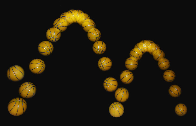
One major use of motion diagrams is the presentation of film through a series of frames taken by a camera; this is sometimes called stroboscopic technique (as seen in ). Viewing an object on a motion diagram allows one to determine whether an object is speeding up or slowing down, or if it is at constant rest. As the frames are taken, we can assume that an object is at a constant rest if it occupies the same position over time. We can assume that an object is speeding up if there is a visible increase in the space between objects as time passes, and that it is slowing down if there is a visible decrease in the space between objects as time passes. The objects on the frame come very close together.

Bouncing Ball: A bouncing ball captured with a stroboscopic flash at 25 images per second.
Key Points
- The four kinematic equations involve five kinematic variables: d,v,v0,a and t.
- Each equation contains only four of the five variables and has a different one missing.
- It is important to choose the equation that contains the three known variables and one unknown variable for each specific situation.
- Motion diagrams represent the motion of an object by displaying its location at various equally spaced times on the same diagram.
- Motion diagrams show an object’s initial position and velocity and presents several spots in the center of the diagram. These spots reveal the object’s state of motion.
- Motion diagrams contain information about an object’s position at particular time instances and is therefore more informative than a path diagram.
Key Terms
- kinematics: The branch of physics concerned with objects in motion.
- stroboscopic: Relating to an instrument used to make a cyclically moving object appear to be slow-moving, or stationary.
- diagram: A graph or chart.
- motion: A change of position with respect to time.
LICENSES AND ATTRIBUTIONS
CC LICENSED CONTENT, SHARED PREVIOUSLY
- Curation and Revision. Provided by: Boundless.com. License: CC BY-SA: Attribution-ShareAlike
CC LICENSED CONTENT, SPECIFIC ATTRIBUTION
- OpenStax College, College Physics. September 17, 2013. Provided by: OpenStax CNX. Located at: http://cnx.org/content/m42125/latest/?collection=col11406/1.7. License: CC BY: Attribution
- kinematics. Provided by: Wiktionary. Located at: en.wiktionary.org/wiki/kinematics. License: CC BY-SA: Attribution-ShareAlike
- Motion diagram. Provided by: Wikipedia. Located at: en.Wikipedia.org/wiki/Motion_diagram. License: CC BY-SA: Attribution-ShareAlike
- motion. Provided by: Wiktionary. Located at: en.wiktionary.org/wiki/motion. License: CC BY-SA: Attribution-ShareAlike
- diagram. Provided by: Wiktionary. Located at: en.wiktionary.org/wiki/diagram. License: CC BY-SA: Attribution-ShareAlike
- stroboscopic. Provided by: Wikipedia. Located at: en.Wikipedia.org/wiki/stroboscopic. License: CC BY-SA: Attribution-ShareAlike
- Boundless. Provided by: Amazon Web Services. Located at: s3.amazonaws.com/figures.boundless.com/51129b2ee4b0c14bf464ce1b/1.jpg. License: CC BY: Attribution
- Provided by: Wikimedia. Located at: http://upload.wikimedia.org/Wikipedia/commons/3/3c/Bouncing_ball_strobe_edit.jpg. License: CC BY: Attribution

