1.4: Spacetime Diagrams
- Page ID
- 43236
\( \newcommand{\vecs}[1]{\overset { \scriptstyle \rightharpoonup} {\mathbf{#1}} } \)
\( \newcommand{\vecd}[1]{\overset{-\!-\!\rightharpoonup}{\vphantom{a}\smash {#1}}} \)
\( \newcommand{\dsum}{\displaystyle\sum\limits} \)
\( \newcommand{\dint}{\displaystyle\int\limits} \)
\( \newcommand{\dlim}{\displaystyle\lim\limits} \)
\( \newcommand{\id}{\mathrm{id}}\) \( \newcommand{\Span}{\mathrm{span}}\)
( \newcommand{\kernel}{\mathrm{null}\,}\) \( \newcommand{\range}{\mathrm{range}\,}\)
\( \newcommand{\RealPart}{\mathrm{Re}}\) \( \newcommand{\ImaginaryPart}{\mathrm{Im}}\)
\( \newcommand{\Argument}{\mathrm{Arg}}\) \( \newcommand{\norm}[1]{\| #1 \|}\)
\( \newcommand{\inner}[2]{\langle #1, #2 \rangle}\)
\( \newcommand{\Span}{\mathrm{span}}\)
\( \newcommand{\id}{\mathrm{id}}\)
\( \newcommand{\Span}{\mathrm{span}}\)
\( \newcommand{\kernel}{\mathrm{null}\,}\)
\( \newcommand{\range}{\mathrm{range}\,}\)
\( \newcommand{\RealPart}{\mathrm{Re}}\)
\( \newcommand{\ImaginaryPart}{\mathrm{Im}}\)
\( \newcommand{\Argument}{\mathrm{Arg}}\)
\( \newcommand{\norm}[1]{\| #1 \|}\)
\( \newcommand{\inner}[2]{\langle #1, #2 \rangle}\)
\( \newcommand{\Span}{\mathrm{span}}\) \( \newcommand{\AA}{\unicode[.8,0]{x212B}}\)
\( \newcommand{\vectorA}[1]{\vec{#1}} % arrow\)
\( \newcommand{\vectorAt}[1]{\vec{\text{#1}}} % arrow\)
\( \newcommand{\vectorB}[1]{\overset { \scriptstyle \rightharpoonup} {\mathbf{#1}} } \)
\( \newcommand{\vectorC}[1]{\textbf{#1}} \)
\( \newcommand{\vectorD}[1]{\overrightarrow{#1}} \)
\( \newcommand{\vectorDt}[1]{\overrightarrow{\text{#1}}} \)
\( \newcommand{\vectE}[1]{\overset{-\!-\!\rightharpoonup}{\vphantom{a}\smash{\mathbf {#1}}}} \)
\( \newcommand{\vecs}[1]{\overset { \scriptstyle \rightharpoonup} {\mathbf{#1}} } \)
\(\newcommand{\longvect}{\overrightarrow}\)
\( \newcommand{\vecd}[1]{\overset{-\!-\!\rightharpoonup}{\vphantom{a}\smash {#1}}} \)
\(\newcommand{\avec}{\mathbf a}\) \(\newcommand{\bvec}{\mathbf b}\) \(\newcommand{\cvec}{\mathbf c}\) \(\newcommand{\dvec}{\mathbf d}\) \(\newcommand{\dtil}{\widetilde{\mathbf d}}\) \(\newcommand{\evec}{\mathbf e}\) \(\newcommand{\fvec}{\mathbf f}\) \(\newcommand{\nvec}{\mathbf n}\) \(\newcommand{\pvec}{\mathbf p}\) \(\newcommand{\qvec}{\mathbf q}\) \(\newcommand{\svec}{\mathbf s}\) \(\newcommand{\tvec}{\mathbf t}\) \(\newcommand{\uvec}{\mathbf u}\) \(\newcommand{\vvec}{\mathbf v}\) \(\newcommand{\wvec}{\mathbf w}\) \(\newcommand{\xvec}{\mathbf x}\) \(\newcommand{\yvec}{\mathbf y}\) \(\newcommand{\zvec}{\mathbf z}\) \(\newcommand{\rvec}{\mathbf r}\) \(\newcommand{\mvec}{\mathbf m}\) \(\newcommand{\zerovec}{\mathbf 0}\) \(\newcommand{\onevec}{\mathbf 1}\) \(\newcommand{\real}{\mathbb R}\) \(\newcommand{\twovec}[2]{\left[\begin{array}{r}#1 \\ #2 \end{array}\right]}\) \(\newcommand{\ctwovec}[2]{\left[\begin{array}{c}#1 \\ #2 \end{array}\right]}\) \(\newcommand{\threevec}[3]{\left[\begin{array}{r}#1 \\ #2 \\ #3 \end{array}\right]}\) \(\newcommand{\cthreevec}[3]{\left[\begin{array}{c}#1 \\ #2 \\ #3 \end{array}\right]}\) \(\newcommand{\fourvec}[4]{\left[\begin{array}{r}#1 \\ #2 \\ #3 \\ #4 \end{array}\right]}\) \(\newcommand{\cfourvec}[4]{\left[\begin{array}{c}#1 \\ #2 \\ #3 \\ #4 \end{array}\right]}\) \(\newcommand{\fivevec}[5]{\left[\begin{array}{r}#1 \\ #2 \\ #3 \\ #4 \\ #5 \\ \end{array}\right]}\) \(\newcommand{\cfivevec}[5]{\left[\begin{array}{c}#1 \\ #2 \\ #3 \\ #4 \\ #5 \\ \end{array}\right]}\) \(\newcommand{\mattwo}[4]{\left[\begin{array}{rr}#1 \amp #2 \\ #3 \amp #4 \\ \end{array}\right]}\) \(\newcommand{\laspan}[1]{\text{Span}\{#1\}}\) \(\newcommand{\bcal}{\cal B}\) \(\newcommand{\ccal}{\cal C}\) \(\newcommand{\scal}{\cal S}\) \(\newcommand{\wcal}{\cal W}\) \(\newcommand{\ecal}{\cal E}\) \(\newcommand{\coords}[2]{\left\{#1\right\}_{#2}}\) \(\newcommand{\gray}[1]{\color{gray}{#1}}\) \(\newcommand{\lgray}[1]{\color{lightgray}{#1}}\) \(\newcommand{\rank}{\operatorname{rank}}\) \(\newcommand{\row}{\text{Row}}\) \(\newcommand{\col}{\text{Col}}\) \(\renewcommand{\row}{\text{Row}}\) \(\newcommand{\nul}{\text{Nul}}\) \(\newcommand{\var}{\text{Var}}\) \(\newcommand{\corr}{\text{corr}}\) \(\newcommand{\len}[1]{\left|#1\right|}\) \(\newcommand{\bbar}{\overline{\bvec}}\) \(\newcommand{\bhat}{\widehat{\bvec}}\) \(\newcommand{\bperp}{\bvec^\perp}\) \(\newcommand{\xhat}{\widehat{\xvec}}\) \(\newcommand{\vhat}{\widehat{\vvec}}\) \(\newcommand{\uhat}{\widehat{\uvec}}\) \(\newcommand{\what}{\widehat{\wvec}}\) \(\newcommand{\Sighat}{\widehat{\Sigma}}\) \(\newcommand{\lt}{<}\) \(\newcommand{\gt}{>}\) \(\newcommand{\amp}{&}\) \(\definecolor{fillinmathshade}{gray}{0.9}\)A spacetime diagram is used for plotting and visualizing events and worldlines.
A worldline is a path through spacetime.
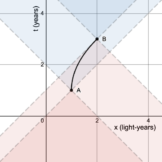
By convention, time is put on the vertical axis of spacetime diagrams, which means that the slope is not equal to the velocity like it is in typical position vs. time graphs. Instead, the slope is equal to the reciprocal of the velocity. An example spacetime diagram is shown in Fig. 1.4.1.

The diagram shows two events, labeled A and B, that are connected by a wordline (solid line) that shows an object that starts at rest and accelerates close to the speed of light. Each event has a pair of lines (dashed lines) that form light cones.
A light cone is formed by the set of all possible wordlines of light that intersect a particular event, and it divides the spacetime into past, future, and elsewhere (causally disconnected).
The blue region above each event represents the set of all causally-connected events that exist in the event's future. The red region below each event represents the set of all causally-connected events that exist in the event's past. Events outside of the light cones are far enough away that even light could not be present at both.
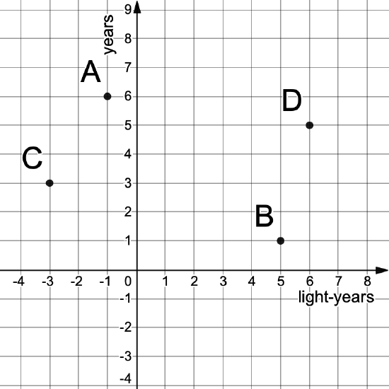
For each of the events in Figure 1.4.2, indicate whether the other events are in the past, future, or elsewhere regions.

Figure \(\PageIndex{2}\): A spacetime diagram with four events indicated.
- Answer
-
For each event, you can draw a pair of lines at 45 degree angles to divide up the space. Events within the light cone and above are in the future, within the light cone and below are in the past, and others are elsewhere.
- Event A: C in the past, all others elsewhere
- Event B: D in the future, all others elsewhere
- Event C: A in the future, all others elsewhere
- Event D: B in the past, all others elsewhere
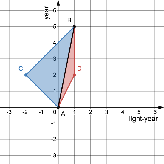
Events A and B are connected by three different wordlines, as shown in Fig. 1.4.3. Calculate the proper time along each worldine (AB, ACB, and ADB).

Figure \(\PageIndex{3}\): Events A and B are connected by three different worldlines.
- Answer
-
We can use the definition of the spacetime interval to calculate the proper time. For worldlines ACB and ADB, we must break the calculation into two separate segments.
For worldline AB:
\[\begin{align*}\Delta \tau_\text{AB}^2&=\Delta t_\text{AB}^2-\Delta x_\text{AB}^2 &&\text{definition of spacetime interval}\\ \Delta \tau_\text{AB}&=\sqrt{\Delta t_\text{AB}^2-\Delta x_\text{AB}^2}&&\text{solve for }\Delta \tau_\text{AB}\\ \Delta \tau_\text{AB}&=\sqrt{(5\text{ year})^2-(1\text{ light-year})^2}&&\text{substitute numbers}\\ \Delta \tau_\text{AB}&=4.90 \text{ years}&&\text{final answer}\end{align*}\]
For wordline ACB:
\[\begin{align*}\Delta \tau_\text{AC}^2&=\Delta t_\text{AC}^2-\Delta x_\text{AC}^2&&\text{definition of spacetime interval}\\ \Delta \tau_\text{AC}&=\sqrt{\Delta t_\text{AC}^2-\Delta x_\text{AC}^2}&&\text{solve for }\Delta \tau_\text{AC}\\ \Delta \tau_\text{AC}&=\sqrt{(2\text{ year})^2-(-2\text{ light-year})^2}&&\text{substitute numbers}\\ \Delta \tau_\text{AC}&=0\text{ years}&&\text{final answer for AC}\end{align*}\]
\[\begin{align*}\Delta \tau_\text{CB}^2&=\Delta t_\text{CB}^2-\Delta x_\text{CB}^2&&\text{definition of spacetime interval}\\ \Delta \tau_\text{CB}&=\sqrt{\Delta t_\text{CB}^2-\Delta x_\text{CB}^2}&&\text{solve for }\Delta \tau_\text{CB}\\ \Delta \tau_\text{CB}&=\sqrt{(3\text{ year})^2-(3\text{ light-year})^2}&&\text{substitute numbers}\\ \Delta \tau_\text{CB}&=0\text{ years}&&\text{final answer for CB}\end{align*}\]
\[\Delta \tau_\text{ACB}=\Delta \tau_\text{AC}+\Delta \tau_\text{CB}=0\text{ years}\nonumber\]
For worldline ADB:
\[\begin{align*}\Delta \tau_\text{AD}^2&=\Delta t_\text{AD}^2-\Delta x_\text{AD}^2&&\text{definition of spacetime interval}\\ \Delta \tau_\text{AD}&=\sqrt{\Delta t_\text{AD}^2-\Delta x_\text{AD}^2}&&\text{solve for }\Delta \tau_\text{AD}\\ \Delta \tau_\text{AD}&=\sqrt{(2\text{ year})^2-(1\text{ light-year})^2}&&\text{substitute numbers}\\ \Delta \tau_\text{AD}&=1.73\text{ years}&&\text{final answer for AD}\end{align*}\]
\[\begin{align*}\Delta \tau_\text{DB}^2&=\Delta t_\text{DB}^2-\Delta x_\text{DB}^2&&\text{definition of spacetime interval}\\ \Delta \tau_\text{DB}&=\sqrt{\Delta t_\text{DB}^2-\Delta x_\text{DB}^2}&&\text{solve for }\Delta \tau_\text{DB}\\ \Delta \tau_\text{DB}&=\sqrt{(3\text{ year})^2-(0\text{ light-year})^2}&&\text{substitute numbers}\\ \Delta \tau_\text{CB}&=3\text{ years}&&\text{final answer for DB}\end{align*}\]
\[\Delta \tau_\text{ADB}=\Delta \tau_\text{AD}+\Delta \tau_\text{DB}=4.73\text{ years}\nonumber\]
In the previous exercise, note that the wordline connecting A and B directly was the one with the greatest proper time. That is also the path that a free particle would follow (i.e. the inertial path). This fact turns out to be true generally, not just for this problem. We call this phenomenon The Principle of Maximal Aging.
Definition: The Principle of Maximal Aging*
The wordline that a free particle would take between two events is the one with the greatest proper time compared to all other wordlines.
*This terminology is borrowed from Exploring Black Holes by Edwin Taylor and John Wheeler.


