2.5: Spacetime Diagrams

In Special Relativity, we constructed light cones using lines at 45 degree angles. One way to understand that is to consider the fact that \(d\tau^2=0\) for light, which we can use to solve for the slope \(\frac{dt}{dx}\).

\[\begin{align*}\cancelto{0}{d\tau^2}&=dt^2-dx^2&&\text{lightlike interval}\\\frac{dt}{dx}&=\pm 1&&\text{solve for }\frac{dt}{dx}\end{align*}\]

Here we see that the slope is +1 or -1 if we use natural units. We can repeat the same process to determine how to sketch light cones on a t-r slice (that is, \(d\theta=d\phi=0\)) using the Schwarzschild metric. The result is

\[\frac{dt}{dr}=\pm\frac{1}{1-\frac{2M}{r}}.\nonumber\]

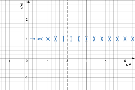
The slopes of the light cones depend on \(r\), as shown in Figure \(\PageIndex{1}\).

Figure \(\PageIndex{1}\): Examples of Schwarzschild light cones. The light cones look like those from Special Relativity for large values of \(r\) but vertically squeeze as \(r\to 2M\). Below \(r=2M\), the light cones squeeze horizontally as \(r\to 0\). Note that the axes have been normalized by the mass \(M\). (Copyright; author via source)

For large values of \(r\), the light cones look like those from Special Relativity. As we approach \(r=2M\) from the outside, the light cones squeeze in the vertical direction, eventually becoming vertical lines right at \(r=2M\). Below \(r=2M\), the light cones squeeze horizontally.

Exercise \(\PageIndex{1}\)

What does the squeezing of the light cones say about the possible futures of particles near \(r=2M\) on the outside?

Answer

If we look at the light cone that is closest to \(r=2M\), we see that there is a very limited range of r-values where the particle could be a short time later. That limited range of r-values gets even more limited the closer you get to \(r=2M\). The result is that the particle cannot pass \(r=2M\).

Exercise \(\PageIndex{2}\)

Light cones divide spacetime into past, future, and elsewhere. In Special Relativity, we saw that past was below, future was above, and elsewhere was on either side. Which regions in Fig. 2.5.1 are elsewhere for \(r<2M\)?

Answer

Let's start by rewriting the Schwarzschild spacetime interval on a t-r slice (i.e. \(d\theta=d\phi=0\)).

\[d\tau^2=\left (1-\frac{2M}{r}\right)dt^2-\frac{1}{1-\frac{2M}{r}}dr^2-r^2\cancelto{0}{d\theta^2}-r^2\sin^2\theta \cancelto{0}{d\phi^2}\nonumber\]

Now consider one of the light cones of Fig. 2.5.1. If we take a small step either directly up or down from one of the vertices, then \(dr=0\). The spacetime interval reduces to

\[d\tau^2=\left(1-\frac{2M}{r}\right)dt^2.\nonumber\]

If \(r<2M\), then \(d\tau^2<0\) and the interval is spacelike, which means that the regions directly above and below the light cone are elsewhere.

If we were instead to take a small step either directly left or right from one of the vertices, then \(dt=0\). The spacetime interval reduces to

\[d\tau^2=-\frac{1}{1-\frac{2M}{r}}dr^2.\nonumber\]

If \(r<2M\), then \(d\tau^2>0\) and the interval is timelike, which means that the regions to the left and right are the future and past.

The bottom line is that the future does not require moving forward in \(t\), but it does require moving to smaller values or \(r\). Inside of \(r=2M\), the roles of the t-coordinate and r-coordinate effectively switch!

The previous examples demonstrate that there is something weird and special about \(r=2M\). Particles on the outside apparently cannot penetrate to the inside, and particles on the inside inevitably end up at \(r=0\). You can also see how the spacetime interval diverges (i.e. becomes undefined) at \(r=2M\). We call this special location the event horizon.

Definition: Event Horizon

In Schwarzschild coordinates, the event horizon is the set of all locations where \(r=2M\). It is one of two locations where the spacetime interval diverges.

For all stars and planets, \(r=2M\) lies well below the surface, which means that this "point of no return" is inaccessible. Black holes, on the other hand, have all of their mass concentrated within the event horizon, which means that the event horizon is accessible.

Note

While the event horizon is a special location, there is nothing physically located there.

There is one more place where the spacetime interval diverges: \(r=0\). This is called the singularity.

Definition: Singularity

The singularity of a black hole is its center, where \(r=0\).

It is difficult to say much about the singularity with confidence. The equations of General Relativity rely on the ability to patch together locally flat references frames, but spacetime is so warped at the singularity that it is not possible to construct a locally flat reference frame there. Is the entire mass of the black hole concentrated at that one single point? Is the singularity a portal to another universe? Is the singularity even a point, as opposed to a small chunk? These are difficult questions to answer.