
1.2: Wave Properties


- Last updated
- Nov 8, 2022
- Save as PDF

( \newcommand{\kernel}{\mathrm{null}\,}\)
Periodic Waves
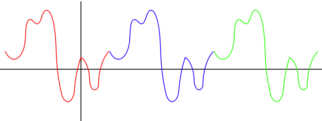
There are qualities that are not required of general waves which are nonetheless common features of waves encountered in nature. The most common special characteristic of a wave is when it continually repeats a specific waveform as it propagates. Such a wave is said to be periodic. There are a couple ways to determine if a wave is periodic. The first is to take a snapshot of the wave, and see if its waveform is repeated in space:
Figure 1.2.1a – Snapshot of a Periodic Wave
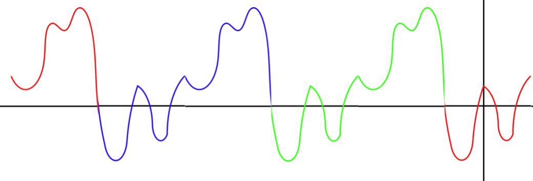
It should be noted that the starting point of each waveform in the diagram above was chosen arbitrarily. That is, if we look at the same snapshot of the wave as above, we could just as easily demonstrate its periodic nature with different segments:
Figure 1.2.1b – Snapshot of a Periodic Wave
The second way to determine if a wave is periodic is mathematical. The function repeats itself upon translation by a certain distance in the \pm x direction. That is:
f\left(x\pm vt\right) = f\left(x\pm vt \pm n \lambda\right),\;\;\;\;\;\;n=0,\;1,\;2,\dots
The quantity \lambda is the length of the repeating waveform, and is called the wavelength of the wave. A glance at the two diagrams above should make it clear that the wavelength is a universal feature of that particular wave, and does not depend upon where we choose the starting point to be.
The snapshot of the wave tells us something about its spatial features, but the wave is moving, so if we want to know something about its time-dependence, we need to select a specific point in space, and observe the displacement of the medium as the wave goes by. The wave moves at a constant speed, and the length of each repeating waveform is the same, so the time span required for a single waveform to go by is a constant for the entire wave, called the period of the wave. An alternative way of measuring the temporal feature of the wave is the rate at which medium displacements repeat, called frequency. Frequency is measured in units of cycles per second, a unit known as hertz (Hz). Since 1 period is the time required for one cycle, there is a simple relationship between these quantities:
f=\dfrac{1}{T}
We can make another association of periodic wave properties. If we pick a specific point on a waveform (called a point of fixed phase for the wave), and follow its motion, it should be clear that it travels a full wavelength in the time of one period. We therefore can relate the wave speed, wavelength, and period (or frequency):
Wave Polarization
While the disturbance is not always a displacement of a medium, it always has a directional element to it. A wave that actually displaces a medium has an obvious direction: that of the displacement. Other waves have directional gradients that signify a direction. The direction in which the pressure is changing fastest (the pressure gradient direction) defines a direction for sound waves, and the direction of the electric field vectors defines a direction for light. This directional aspect of waves is also given a name: polarization. Generally the direction of medium displacement or gradient is compared to the direction of the wave's motion. There are two special cases that we will encounter for polarization of a wave:
transverse polarization: the medium's displacement or gradient is perpendicular to the wave’s direction of motion
Figure 1.2.2 – Transverse Wave
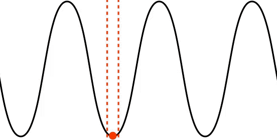
Note that the displacement of a single point in the medium (depicted by the red dot) is moving only vertically, while the wave moves horizontally. That these two motions are perpendicular to each other is the defining characteristic of a transversely polarized wave. Waves on strings and surface water waves are examples of this kind of wave. As noted earlier, not all waves involve the medium displacing (we will see some examples where this is the case later), but whatever fluctuation is occurring has a direction that can be compared with the direction of the wave's motion.
longitudinal polarization: the medium's displacement or gradient is parallel to the wave’s direction of motion.
Figure 1.2.3 – Longitudinal Wave
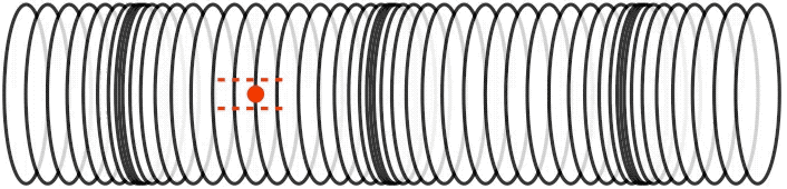
This time the displacement of a single point in the medium is parallel to the direction of the motion of the wave, the defining characteristic of a longitudinally polarized wave. Notice that like any other wave, the medium is not traveling with the wave, it is moving back-and forth. Physically these are waves induced by compressions (regions where the medium is more dense) and rarefactions (regions where the medium is less dense). These kinds of waves can be created in springs (as depicted above), but the most common physical example of this kind of wave is sound. Any medium (solid, liquid, or gas) will react to compression, and will therefore exhibit this kind of wave.
Alert
Snapshot graphs of waves of both kinds of polarization are sketched graphically with the displacement on the vertical axis and the position on the horizontal axis. When this is done, it "looks like" a transverse wave, but it is important to keep in mind that such a graph is not a picture of the wave. The vertical axis measures the displacement of the medium from the equilibrium point, which in the case of the red dot on the spring coil for the longitudinal wave in Figure 1.2.3 is the center of the horizontal dotted red lines.
Harmonic Waves
In the category of periodic waves, the easiest to work with mathematically are harmonic waves. The word "harmonic" is basically synonymous with "sinusoidal." For a one-dimensional wave, one might therefore assume that a harmonic wave function looks like:
f\left(x,t\right) = A\cos\left(x\pm vt\right)
While this comes close, it has a problem with units. The total phase of the wave function (the part in parentheses that is the argument of the cosine) cannot have any physical units, and this function has a phase with units of length. We can therefore repair this problem by dividing the phase by a constant of the wave that has units of length. The obvious such constant is the wavelength. So now our candidate wave function is:
f\left(x,t\right) = A\cos\left[\frac{1}{\lambda}\left(x\pm vt\right)\right]
This gets close, but if we are using radians as the measurement of phase, there is one more change we must add. If we consider a snapshot of this wave at t=0, we would find that the sinusoidal waveform should repeat itself every time the value of x is displaced by \lambda. If we are using radians as our angular measure, then this requires multiplying the phase by 2\pi. Then every change of x by \lambda will result in a change in the phase by 2\pi, and the function repeats itself properly. So we now have:
f\left(x,t\right) = A\cos\left[\frac{2\pi}{\lambda}\left(x\pm vt\right)\right]
There is one final addition to the phase that we need to make. Suppose we take a snapshot of the wave at t=0 and look at the origin, x=0. This function tells us that the value of the wave's displacement must be its maximum: A. This is not a very general wave! To account for the possibility that the wave might have a different initial condition at the origin, we need to include a phase constant, \phi. Distributing the factor of \frac{2\pi}{\lambda}, and using Equation 1.2.3, we get the final form of the wave function of a 1-dimensional harmonic wave:
f\left(x,t\right) = A\cos\left(\frac{2\pi}{\lambda}x\pm \frac{2\pi}{T}t + \phi\right)
It is common to write this wave function in more compact ways. The first involves the definition of the wave number k, and angular frequency \omega:
k\equiv \frac{2\pi}{\lambda},\;\;\; \omega\equiv 2\pi f=\frac{2\pi}{T} \;\;\;\Rightarrow\;\;\;f\left(x,t\right) = A\cos\left(kx\pm \omega t + \phi\right)
Another definition that saves even more space is lumping the total phase of the wave into a single function variable: \Phi\left(x,t\right). It is clearly linear in the variables x and t. That is:
Finally, it should be noted that although the cosine function was arbitrarily chosen here, we could have just as easily chose a sine function. The only difference between representing the wave with these two functions is the phase constant. That is, we can change from one function to the other if we change the phase constant by \frac{\pi}{2}:
\cos\left(\Phi\right)=\sin\left(\Phi + \frac{\pi}{2}\right)\;\;\;\Rightarrow\;\;\; \phi\rightarrow\phi+\frac{\pi}{2}
Wave Graphs
The important thing to take away from the harmonic wave function in Equation 1.2.7 is that the wave has four constants of the motion that completely define it. Besides the wavelength, period, and phase constant, there is the amplitude, A. All of these remain fixed in time, completely defining the wave that evolves thanks to its x and t dependence. It is often useful to use these constants to analyze a wave in parts. For example, we have already discussed analyzing the spatial features of the wave by taking a "snapshot" – a frozen moment in time. This amounts to choosing a value for t (often zero, but not always), so that the wave function now becomes only a function of x.
We can also isolate the time variable. In this case, we pick a specific position x, and graph the time dependence of the displacement of that point in the wave. For harmonic waves, these displacement-vs-time graphs represent harmonic oscillation. It should be noted that like the spatial graph, the time graph is a cosine (or sine) function, and this can lead to confusion, as it "looks like" a wave.
What links these two graphs is the motion of the wave. The speed of the wave is related to the wavelength (which can be read off the position graph) and the period (which can be read off the time graph). The direction of the wave's motion gives us the relative signs of the position and time variables in the wave function (recall that opposite signs means it is moving in the +x-direction). Determining the phase constant requires understanding the meaning of "total phase," and some simple algebra. Let's see how this all fits together with an example.
Example \PageIndex{1}
The figure below is a graph of the simple harmonic motion of a particle of string through which an harmonic transverse wave is passing (the displacement is parallel to the y-axis, and the motion is along the x-axis). The position (x-value) of the oscillating particle is 5m, as indicated on the graph.

- One of the four position graphs given below represents a snap-shot of the wave at a given instant in time (the moment in time for each case is indicated on the graph). Find the y-vs-x graph below that belongs to this wave.

- Find the amplitude, wavelength and period of this wave.
- Find the speed at which this wave is traveling.
- Find the direction (\pm x) in which this wave is moving.
- Find the phase constant in the range [0, 2\pi] for the wave function of this wave.
- Solution
-
a. The one thing that both graphs have in common is the displacement of the particle of string. The harmonic motion graph occurs at the position x=5m, so we can look at what displacement the four prospective graphs give for that position at a common time. Let's start with graph A. The value of the displacement at the position x=5m of the particle is y=-2, and this occurs at time t=2s. Looking back at the harmonic motion graph, we see that the displacement of the particle at t=2s is y=0, so graph A cannot represent the same wave as the harmonic motion graph. Graph B has a displacement of y=-1 at time t=3s. Looking back at the harmonic motion graph, we see that at t=3s the displacement is between y=+1 and y=+2, so graph B also does not work. Graph C has a displacement at x=5m, t=2s that matches that of the harmonic motion graph (i.e. y=0). It's easy to confirm using the logic shown above that graph D does not work, so the answer is graph C. It is important to note that graph C is by no means unique, it is simply the only one that works from the four choices given. But now that we know graph C represents this wave, we know significantly more about it, and we will use this information for the remaining parts of this example.
b. The maximum displacement of the string is the amplitude of the wave, and both graphs must agree on this. They do, and it is a value of 2 (units are not given). We know that graph C is a proper snapshot graph of this wave, which makes the distance between peaks equal to the wavelength, so \lambda=4m. The time interval between peaks on the harmonic motion graph is the period of one oscillation, so T=8s.
c. With the wavelength and period, we can immediately compute the wave speed: v=\frac{\lambda}{T} = 0.5\frac{m}{s}.
d. Now things start to get a bit tricky, and a little visualization & logic are required. The one point we know about from these two graphs is x=5m, t=2s. Now let's consider what happens to that particle of string a short time later. On the harmonic motion graph, we see that if we move to a slightly larger value of t, the displacement becomes positive. The wave must therefore moving in a direction such that a short time later the displacement will rise. Looking at the snapshot of the wave in graph C, we see that the direction we need to shift the wave form such that the displacement immediately starts going up is the -x-direction. The wave must therefore be moving in that direction. Note that if the common point between the two graphs happened to be a maximum or minimum of the wave, then it would not be possible to determine the direction of the wave velocity, because the displacement a short time later would be in the same direction no matter which way the wave was moving.
e. First, it should be noted that there are an infinite number of phase constants, since one can always add or subtract 2\pi to get a new phase constant that will also work. So our task here is to find any phase constant that works, then add or subtract an appropriate number of units of 2\pi to get a value that falls within the range required. To solve for a phase constant, one must first understand what the total phase of the wave is. Given that we are using a cosine function, we know that the peak of the wave occurs when the argument of the cosine (i.e. the total phase) is an integer multiplied by 2\pi. We will make it easy on ourselves by just choosing zero. So we need to find a position and time for which the displacement of the wave is a maximum – any choice will work, and as an exercise, the reader should try more points to prove this. For this solution, we will use the peak on the harmonic motion graph at x=5m, t=4s. Note that we must choose the x and t terms to have the same sign, as we know the wave is moving in the -x-direction. We will choose both to have positive signs, but both negative will also work.
\Phi\left(x,t\right)=\frac{2\pi}{\lambda}x\pm \frac{2\pi}{T}t +\phi\;\;\; \Rightarrow\;\;\; 0=\frac{2\pi}{4m}\left(5m\right)+ \frac{2\pi}{8s}\left(4s\right) +\phi\;\;\; \Rightarrow\;\;\;\phi=-\frac{7}{2}\pi\nonumber
This phase constant doesn't fall within the desired [0, 2\pi] range, so we add 4\pi to it and find \phi=\frac{\pi}{2}.
Wave Velocity
Up until now, we have simply stated that waves have fixed velocities. What we have not yet considered are the physical conditions that determine the speed that a wave will have. Clearly these conditions must depend only upon the type of wave it is (string, slinky, light, sound, etc.) and the medium through which it is passing. We will use our tools from classical mechanics to look at the simple physical physical system of a transverse wave traveling through a taut string.
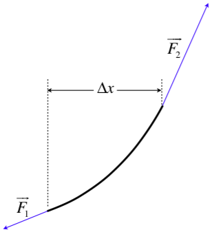
The wave function describes the displacement of a single particle of the string, so we will start with a small segment. The wave form curves the string, so the pulls of tension from each end of an infinitesimal segment of the string are not directly opposite to each other. A free-body diagram of such a segment of length \Delta x (the bend is exaggerated for the purpose of illustration) looks like this (note that we are ignoring gravity here):
Figure 1.2.4a – Free-Body Diagram of a Segment of String
The two forces can now be broken into horizontal and vertical components.
Figure 1.2.4b – Free-Body Diagram of a Segment of String
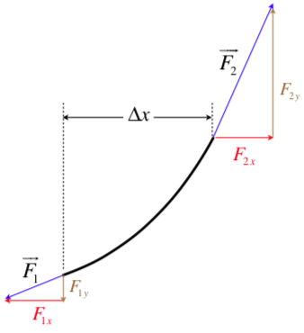
Remember that this is a transverse wave, which means that this segment only accelerates vertically. The horizontal components of the forces therefore must cancel, and remain fixed – the magnitude of the horizontal components must therefore be the constant horizontal tension applied to the string.
\text{tension} = F = F_{1x} = F_{2x}
Now apply Newton's 2nd law in the vertical direction. Setting up as the positive direction, we have:
F_{2y} - F_{1y} = ma_y
The mass of this segment of string is the linear mass density of the string (which we will call \mu) multiplied by the segment's length \Delta x. The vertical acceleration is the second derivative of the y position with respect to time. Putting these into the equation gives:
F_{2y} - F_{1y} = \left(\mu \Delta x\right)\left(\dfrac{\partial^2y}{\partial t^2}\right)
The two forces \overrightarrow F_1 and \overrightarrow F_2 are pulling directly through the string, so their directions are tangent to the curve made by the string on each end. The slope of the curve made by the string is the first derivative of the displacement with respect to x, and this slope is also the ratio of the vertical force to the horizontal force, so:
\left. \begin{array}{l} \text{slope at bottom of segment:} && \left(\dfrac{\partial y}{\partial x}\right)_1=\dfrac{F_{1y}}{F_{1x}}=\dfrac{F_{1y}}{F} \\ \text{slope at btop of segment:} && \left(\dfrac{\partial y}{\partial x}\right)_2=\dfrac{F_{2y}}{F_{2x}}=\dfrac{F_{2y}}{F} \end{array}\right\} \;\;\; \Rightarrow \;\;\; F_{2y} - F_{1y} = F\left[\left(\dfrac{\partial y}{\partial x}\right)_2-\left(\dfrac{\partial y}{\partial x}\right)_1\right]
Plugging this back into Equation 1.2.12, we get:
F\left[\left(\dfrac{\partial y}{\partial x}\right)_2-\left(\dfrac{\partial y}{\partial x}\right)_1\right]=\mu \Delta x\left(\dfrac{\partial^2y}{\partial t^2}\right)\;\;\; \Rightarrow \;\;\; \dfrac{\left(\dfrac{\partial y}{\partial x}\right)_2-\left(\dfrac{\partial y}{\partial x}\right)_1}{\Delta x}=\dfrac{\mu}{F}\left(\dfrac{\partial^2y}{\partial t^2}\right)
When we require that \Delta x be very small, the left-hand side of the equation becomes a derivative. There is already on derivative, so the result is a second derivative, giving:
\dfrac{\partial^2y}{\partial x^2} = \left(\dfrac{\mu}{F}\right)\dfrac{\partial^2y}{\partial t^2}
But this is precisely the wave equation! So we can just read-off the velocity of the wave (recall from Equation 1.1.3 that the coefficient of the second derivative in time is \frac{1}{v^2}):
\frac{1}{v^2} = \dfrac{\mu}{F} \;\;\; \Rightarrow \;\;\; v=\sqrt{\dfrac{F}{\mu}}
Mechanical Wave Speeds in Other Media
Although we derived the result for the very specific case of a taut string, its general features applies to all mechanical waves – there is always an element of the restoring force in the medium (in the string case, the tension), and the inertial of the medium (in the string case, the linear density), and the square root dependence comes out to be universal as well!
We said in Physics 9A that particles near each other (whether a solid, liquid or gas) exert restoring forces on each other (repel when they get closer, attract when they separate). This force ultimately is what is responsible for the wave speed for which we found the simplest case above, described in terms of tension. If such a wave (which, unlike a transverse string wave, is actually a longitudinal compression wave, and goes by the more generic name of "sound") is traveling through a fluid (defined as either a gas or a liquid), then the Van der Waals restoring forces between the particles are summarized in terms of a quantity called the bulk modulus. The "inertia" part of the wave speed equation changes from the linear mass density of the (one-dimensional) string to the volume mass density of the (three-dimensional) fluid, making the velocity relation look like:
v_{in\;fluid} = \sqrt{\dfrac{B}{\rho}}
It turns out that this bulk modulus depends not only on the makeup of the fluid, but also its temperature. We won't go into any more detail than this about this physical property of fluids.
These compression waves can also travel through solids, and the Van der Waals restoring forces between particles manifest slightly differently than for fluids (as you can imagine, the "spring constants" between nearby particles in a solid are significantly higher than between particles in a fluid). In this case, the physical property that accounts for the restoring force between particles is called Young’s modulus. But the resulting wave speed formula looks the same:
v_{in\;solid} = \sqrt{\dfrac{Y}{\rho}}
We will not explore the exact nature of the bulk and Young's moduli, other than to note that they must obviously have the same units. Simply knowing that they play the same role for fluids and solids respectively as the tension plays for a transverse wave on a string will suffice for our purposes.
Digression: Tsunamis
When one reads above "waves in a fluid", one might be inclined to visualize transverse waves, as one sees on the surface of the ocean. But those waves have as their restoring forces gravity and upward pressure. In fact, such surfable waves are known as "gravity waves" (not to be confused with "gravitational waves" which are themselves very different). The waves-through-fluid for which the equation above applies are longitudinal – like a wave on a slinky that compresses and expands the rings. Such waves in the ocean are significantly faster than their gravity wave counterparts. In cases where an underwater earthquake strikes, a great deal of energy can be transmitted into this type of wave, and its high rate of speed can correspond to quite a long wavelength. When such a wave reaches a beach, the longitudinal displacement of the water can therefore be quite large, vacating the water just offshore for several hundred yards, followed by an expansion onshore a similar distance, inundating the land near the beach. These waves are what are known as tsunamis. These are sometimes mistakenly referred to as "tidal waves", but gravitational effects from the sun and moon are responsible for the tides, and these don't play a role in this type of wave. Also, some visualize tsunamis as very tall waves that crash on shore, but again, tsunamis are longitudinal, so their large displacements are horizontal, not vertical.
Summary of Wave Attributes
To conclude this section, we will recap the wave attributes we have seen so far. For a wave to occur, two things are needed – a medium through which the wave passes, and a "driver" which is the initial source of the energy carried by the wave. Let's look at how each of the wave attributes links to these ingredients.
- wave speed – We just showed above that the speed of the wave depends entirely upon the medium alone. There is no way to generate the wave at its origin such that it will move faster. While we have only shown this for transverse string waves, it is true in general for all waves.
- amplitude – The maximum displacement of an harmonic wave depends upon how much the driver displaces the medium at the source of the wave. We also found that the amplitude can change (get smaller) when the wave is radiating outward from a point source in 2 or 3 dimensions.
- period (or frequency) – The period of the wave is determined by how long it takes the wave's generator to complete a full cycle. The wave's frequency will exactly mimic the frequency at which it is driven.
- wavelength – The length of a wave is determined by a combination of its frequency and wave speed. So we cannot point to either the driver or the medium as the direct cause of wavelength. In some sense, wavelength is a "dependent variable," while the independent variables that we can control from outside are wave speed and frequency.
- polarization – The displacement of the medium can be perpendicular to the wave motion (transverse) or parallel to it (longitudinal).
Example \PageIndex{2}
The transverse harmonic waves carried on a taut string can be adjusted in three ways:
- the tension in the string can be increased or decreased
- the maximum displacement of the driver can be made larger or smaller
- the frequency of oscillation of the driver can be increased or decreased
After a lot of careful adjustments, a wave is created which has the property that the speed of the wave equals the maximum speed that a tiny segment of the string has as the wave passes through it.
- Describe what kinds of changes to the output of the driver (if any) will maintain the equal-speed property above.
- Find the ratio of the amplitude of the wave and its wavelength.
- Solution
-
a. We start with the wave function:
f\left(x,t\right) = A\cos\left(\frac{2\pi}{\lambda}x \pm \frac{2\pi}{T}t+\phi\right)\nonumber
This describes the vertical position of a segment of string as a function of the horizontal position and time. The speed of this segment is therefore the first derivative of this function with respect to time:
v_{string}\left(x,t\right) = \frac{\partial}{\partial t}f\left(x,t\right) = \frac{\partial}{\partial t}A\cos\left(\frac{2\pi}{\lambda}x \pm \frac{2\pi}{T}t+\phi\right) = \mp\frac{2\pi}{T}A\sin\left(\frac{2\pi}{\lambda}x \pm \frac{2\pi}{T}t+\phi\right)\nonumber
The maximum value of the sine function is 1, so the maximum speed of the string is \frac{2\pi}{T}A. In terms of the frequency, this maximum speed is 2\pi fA. We can adjust both the frequency and the amplitude of the driver, and this won't change the speed of the wave (that can only be changed by altering the tension), so for the max speed of the string to remain unchanged (and equal to the wave speed), the amplitude and frequency have to be changed by the same factor, one of them up and the other down.
b. The wavelength can be determined from the speed of the wave and the frequency. The speed of the wave equals the maximum speed of the string, so:
\lambda f = v_{wave} = v_{max\;of\;string} = 2\pi fA \;\;\; \Rightarrow \;\;\; \dfrac{A}{\lambda} = \dfrac{1}{2\pi} \nonumber
Video Lecture
