1.1: Wave Mathematics

Definition of a Wave

A wave is a disturbance that propagates through space at a constant speed. With one notable exception that we will encounter later, this "disturbance" consists of a fluctuation in the ambient condition of a medium. Waves in one dimension maintain a consistent waveform as they propagate (later we will see why this is not so for waves in two and three dimensions). Let's see how we can model this mathematically. We'll start with a localized disturbance frozen in time (think of it as a snapshot) that we describe with a function \(f\left(x\right)\):

Figure 1.1.1 – Snapshot of a Wave

This is the waveform, but to be a wave, it needs to be propagating along the \(x\)-axis, which would make it a function of both \(x\) and \(t\). To turn it into such a function, we first have to think about how a function can be shifted along the \(x\)-axis. This is accomplished by replacing \(x\) in the argument of the function with the sum or difference of \(x\) and the value of the shift. If one wishes to shift the function \(f\left(x\right)\) in the \(+x\) direction by a distance \(a\), then the proper change is to the function \(f\left(x-a\right)\). Note that subtracting \(a\) in the argument shifts the function in the positive \(x\) direction, and adding the constant shifts it in the negative \(x\) direction. We insist that the wave moves at a constant speed, so we want the wave form to shift by the same distance every time the same time interval passes. We therefore have that the general form of a wave function is:

\[f\left(x,t\right)=f\left(x\pm vt\right)\]

This represents a waveform \(f\left(x\right)\) propagating in the \(\mp x\) direction with a speed \(v\).

There are countless functions of \(x\) and \(t\) that we can come up with, but not all can be written in the form described above. When faced with an arbitrary function of \(x\) and \(t\), it can be challenging to determine whether the function represents a wave.

Example \(\PageIndex{1}\)

Determine which (if any) of the functions below represent a traveling wave. For those that do, determine the direction of their propagation, and their speed. In every case the constants \(\alpha\) and \(\beta\) are positive numbers.

1. \(f\left(x,t\right)=\left(1-\alpha x+\beta t\right)^3+\left(2+\alpha x-\beta t\right)^5\)
2. \(f\left(x,t\right)=\sin\left[\left(\alpha x\right)^2-\left(\beta t\right)^2\right]\)
3. \(f\left(x,t\right)=e^{-\alpha x}e^{-\beta t}\)

Solution

The idea here is to do whatever algebra that is necessary to get the function into the form \(f\left(x\pm vt\right)\)...

a. If we factor \(-\alpha^3\) out of the first term, and \(\alpha^5\) out of the second term, we have:

\[f\left(x,t\right)=-\alpha^3\left(-\frac{1}{\alpha}+ \left(x-\frac{\beta}{\alpha} t\right)\right)^3+\alpha^5\left(\frac{2}{\alpha}+ \left(x-\frac{\beta}{\alpha} t\right)\right)^5 \nonumber\]

We can see that this is purely a function of \(\left(x-\frac{\beta}{\alpha} t\right)\). In such problems, it might help to substitute \(z\) for \(\left(x\pm vt\right)\) and show that there are no \(x\)'s or \(t\)'s left over. The resulting function \(f\left(z\right)\) is in fact the waveform. For this case:

\[f\left(z\right)=\left(1-\alpha z\right)^3+\left(2+ \alpha z\right)^5 \nonumber\]

This is therefore a traveling wave moving in the \(+x\) direction (because of the opposite signs of \(x\) and \(t\)), and the speed must be \(\frac{\beta}{\alpha}\).

b. At first glance this might appear to be the function of a traveling wave, but we can show that in fact it cannot be written in the correct form. Writing the difference of two squares as a product gives:

\[f\left(x,t\right)=\sin\left[\left(\alpha x+\beta t\right)\left(\alpha x-\beta t\right)\right]\nonumber\]

Each of the factors has the right form (once a factor of \(\alpha\) is divided out), but if we substitute \(z\) for one of them, we cannot similarly eliminate the second factor. Put another way, one of the factors indicates the wave is moving in the \(+x\) direction, while the other indicates it is moving the opposite way. It can't be doing both, so this is not the equation of a traveling wave.

c. Combining the exponentials gives:

\[f\left(x,t\right)=e^{-\alpha x-\beta t}=e^{-\alpha \left(x+\frac{\beta}{\alpha} t\right)}\;\;\;\Rightarrow\;\;\; f\left(z\right)=e^{-\alpha z}\nonumber\]

Clearly this represents a wave propagating in the \(-x\) direction with a speed of \(\frac{\beta}{\alpha}\).

The Wave Equation

It seems like there has to be an easier way to determine if a function of \(x\) and \(t\) represents a wave. It turns out that there is! To see this, let's start with the basic definition above. If we define \(g_{\pm}\left(x,t\right)\equiv x\pm vt\), then we can write the wave function as \(f\left(g_{\pm}\right)\). Now we can write derivatives of the function with respect to \(x\) and \(t\) in terms of derivatives with respect to \(g_{\pm}\) using the chain rule. Note that these are functions of more than one variable, so we need to use partial derivatives. These work precisely like ordinary derivatives, except that when the derivative is taken with respect to one variable, all the other variables are treated as constants.

\[\begin{array}{l} \dfrac{\partial f}{\partial x}=\dfrac{\partial f}{\partial g_{\pm}}\dfrac{\partial g_{\pm}}{\partial x}=\dfrac{\partial f}{\partial g_{\pm}} && \Rightarrow && \dfrac{\partial^2 f}{\partial x^2}=\dfrac{\partial^2 f}{\partial g_{\pm}^2} \\ \dfrac{\partial f}{\partial t}=\dfrac{\partial f}{\partial g_{\pm}}\dfrac{\partial g_{\pm}}{\partial t}=\pm v\dfrac{\partial f}{\partial g_{\pm}} && \Rightarrow && \dfrac{\partial^2 f}{\partial t^2}= v^2\dfrac{\partial^2 f}{\partial g_{\pm}^2} \end{array}\]

Putting these together gives us a relation between second derivatives known as the wave equation:

\[\dfrac{\partial^2 f}{\partial x^2}=\dfrac{1}{v^2}\dfrac{\partial^2 f}{\partial t^2} \]

This second order partial differential equation holds if and only if the function behaves like a traveling wave (or a linear combination of traveling waves) with speed \(v\).

Example \(\PageIndex{2}\)

For the functions in the previous example, demonstrate whether they do or do not satisfy the wave equation with the proper wave speed.

Solution

We found that the formulas for cases (a) and (c) represent waves, so we plug those into the wave equation:

(a)

\[\dfrac{\partial^2}{\partial x^2}f\left(x,t\right) =\dfrac{\partial^2}{\partial x^2}\left[\left(1-\alpha x+\beta t\right)^3+\left(2+\alpha x-\beta t\right)^5\right] = \dfrac{\partial}{\partial x}\left[-3\alpha\left(1-\alpha x+\beta t\right)^2+5\alpha\left(2+\alpha x-\beta t\right)^4\right] = 6\alpha^2\left(1-\alpha x+\beta t\right)+20\alpha^2\left(2+\alpha x-\beta t\right)^3\nonumber\]

\[\dfrac{\partial^2}{\partial t^2}f\left(x,t\right)=\dfrac{\partial^2}{\partial t^2}\left[\left(1-\alpha x+\beta t\right)^3+\left(2+\alpha x-\beta t\right)^5\right] = \dfrac{\partial}{\partial t}\left[3\beta\left(1-\alpha x+\beta t\right)^2-5\beta\left(2+\alpha x-\beta t\right)^4\right] = 6\beta^2\left(1-\alpha x+\beta t\right)+20\beta^2\left(2+\alpha x-\beta t\right)^3\nonumber\]

From direct comparison, it is clear that these two terms are proportional, which means they satisfy the wave equation:

\[\dfrac{\partial^2}{\partial x^2}f\left(x,t\right) = \frac{\alpha^2}{\beta^2}\dfrac{\partial^2}{\partial t^2}f\left(x,t\right)\nonumber\]

The constant of proportionality for the wave equation is \(\frac{1}{v^2}\), so this confirms that \(v=\frac{\beta}{\alpha}\).

(b)

\[\dfrac{\partial^2}{\partial x^2}f\left(x,t\right) = \dfrac{\partial^2}{\partial x^2}\sin\left[\left(\alpha x\right)^2-\left(\beta t\right)^2\right] = \dfrac{\partial}{\partial x}\left\{2\alpha^2 x\cos\left[\left(\alpha x\right)^2-\left(\beta t\right)^2\right]\right\}=2\alpha^2 \cos\left[\left(\alpha x\right)^2-\left(\beta t\right)^2\right]-4\alpha^4 x^2 \sin\left[\left(\alpha x\right)^2-\left(\beta t\right)^2\right]\nonumber\]

\[\dfrac{\partial^2}{\partial t^2}f\left(x,t\right) = \dfrac{\partial^2}{\partial t^2}\sin\left[\left(\alpha x\right)^2-\left(\beta t\right)^2\right] = \dfrac{\partial}{\partial t}\left\{-2\beta^2 t\cos\left[\left(\alpha x\right)^2-\left(\beta t\right)^2\right]\right\}=-2\beta^2 \cos\left[\left(\alpha x\right)^2-\left(\beta t\right)^2\right]-4\beta^4 t^2 \sin\left[\left(\alpha x\right)^2-\left(\beta t\right)^2\right]\nonumber\]

These two terms are clearly not proportional, so this function does not satisfy the wave equation.

(c)

\[\dfrac{\partial^2}{\partial x^2}f\left(x,t\right) = \dfrac{\partial^2}{\partial x^2}\left[e^{-\alpha x}e^{-\beta t}\right] = \dfrac{\partial}{\partial x}\left[-\alpha e^{-\alpha x}e^{-\beta t}\right] = \alpha^2 e^{-\alpha x}e^{-\beta t}\nonumber\]

\[\dfrac{\partial^2}{\partial t^2}f\left(x,t\right) = \dfrac{\partial^2}{\partial t^2}\left[e^{-\alpha x}e^{-\beta t}\right] = \dfrac{\partial}{\partial t}\left[-\beta e^{-\alpha x}e^{-\beta t}\right] = \beta^2 e^{-\alpha x}e^{-\beta t}\nonumber\]

These two terms are proportional, and the constant of proportionality gives the correct velocity once again.

Waves in Two and Three Dimensions

Consider a two-dimensional wave, such as a ripple radiating outward from a pebble dropped into a still lake. If the distance of the wave front from the source is \(r\), following the "wave form remains unchanged" prescription, the functional form of the traveling wave is \(f\left(r,t\right)=f\left(r-vt\right)\). Alternatively, we can extend the wave equation to two or three dimensions as follows:

\[\begin{array}{l} two\;dimensions: && \dfrac{\partial^2 f}{\partial x^2}+\dfrac{\partial^2 f}{\partial y^2}=\dfrac{1}{v^2}\dfrac{\partial^2 f}{\partial t^2} \\ three\;dimensions: && \dfrac{\partial^2 f}{\partial x^2}+\dfrac{\partial^2 f}{\partial y^2}+\dfrac{\partial^2 f}{\partial z^2}=\dfrac{1}{v^2}\dfrac{\partial^2 f}{\partial t^2} \end{array}\]

In the one-dimensional case, we showed above that the wave form that remains unchanged as it propagates is described by a function that satisfies the wave equation. It turns out that in the two-dimensional case, this is no longer true. We can show this by repeating the procedure outlined in Equation 1.1.2. A waveform that remains unchanged as it spreads radially outward would have the form \(f\left(r,t\right)=f\left(r-vt\right)\) (we are considering an outgoing waveform, which accounts for the minus sign). Defining the function \(g\left(r,t\right)\equiv r - vt\), we have for the derivative of the wave function with respect to \(x\):

\[\dfrac{\partial f}{\partial x}=\left(\dfrac{\partial f}{\partial g}\right)\left(\dfrac{\partial g}{\partial x}\right)=\left(\dfrac{\partial f}{\partial g}\right)\left(\dfrac{\partial g}{\partial r}\right)\left(\dfrac{\partial r}{\partial x}\right)\]

Note that the variable \(r\) depends upon both \(x\) and \(y\), specifically:

\[r=\sqrt{x^2+y^2}=\left(x^2+y^2\right)^{\frac{1}{2}}\;\;\; \Rightarrow \;\;\; \dfrac{\partial r}{\partial x} = \frac{1}{2}\left(x^2+y^2\right)^{-\frac{1}{2}}\left(2x\right) = \dfrac{x}{r},\;\;\;\text{and}\;\;\;\dfrac{\partial r}{\partial y} =\dfrac{y}{r}\]

Plugging this and \(\dfrac{\partial g}{\partial r} = 1\) in above gives:

\[\begin{array}{l} \dfrac{\partial f}{\partial x}=\dfrac{\partial f}{\partial g}\left(\dfrac{x}{r}\right) && \Rightarrow && \dfrac{\partial^2 f}{\partial x^2}=\dfrac{\partial^2 f}{\partial g^2}\left(\dfrac{x^2}{r^2}\right)+\dfrac{\partial f}{\partial g}\left(\dfrac{1}{r}\right)\left(1-\dfrac{x^2}{r^2}\right) \\ \dfrac{\partial f}{\partial y}=\dfrac{\partial f}{\partial g}\left(\dfrac{y}{r}\right) && \Rightarrow && \dfrac{\partial^2 f}{\partial y^2}=\dfrac{\partial^2 f}{\partial g^2}\left(\dfrac{y^2}{r^2}\right)+\dfrac{\partial f}{\partial g}\left(\dfrac{1}{r}\right)\left(1-\dfrac{y^2}{r^2}\right) \end{array}\]

The dependence on \(t\) is the same as in the one-dimensional case:

\[\dfrac{\partial f}{\partial g}=-\dfrac{1}{v}\dfrac{\partial f}{\partial t}\;\;\;\Rightarrow\;\;\;\dfrac{\partial^2 f}{\partial g^2}=\dfrac{1}{v^2}\dfrac{\partial^2 f}{\partial t^2}\]

Plugging this into the previous equations, and adding them together gives:

\[\dfrac{\partial^2 f}{\partial x^2}+\dfrac{\partial^2 f}{\partial y^2}=\dfrac{1}{v^2}\dfrac{\partial^2 f}{\partial t^2}\left(\dfrac{x^2}{r^2}+\dfrac{y^2}{r^2}\right)-\dfrac{1}{v}\dfrac{\partial f}{\partial t}\left(\dfrac{1}{r}\right)\left(2-\dfrac{x^2}{r^2}-\dfrac{y^2}{r^2}\right)\]

Noting that \(x^2+y^2=r^2\), we finally get:

\[\dfrac{\partial^2 f}{\partial x^2}+\dfrac{\partial^2 f}{\partial y^2}=\dfrac{1}{v^2}\dfrac{\partial^2 f}{\partial t^2}-\dfrac{1}{v}\dfrac{\partial f}{\partial t}\left(\dfrac{1}{r}\right)\]

The second term on the right hand side of the equation clearly makes this differential equation look different from the one-dimensional wave equation. So the question is, which is the correct way of describing a two-dimensional wave? Does it maintain its wave form as it propagates outward, or does it satisfy our previous wave equation extended to two dimensions? The figures below display the two possibilities we are talking about.

Figure 1.1.2 – Two-Dimensional Circularly-Radiating Function with Unchanging Waveform

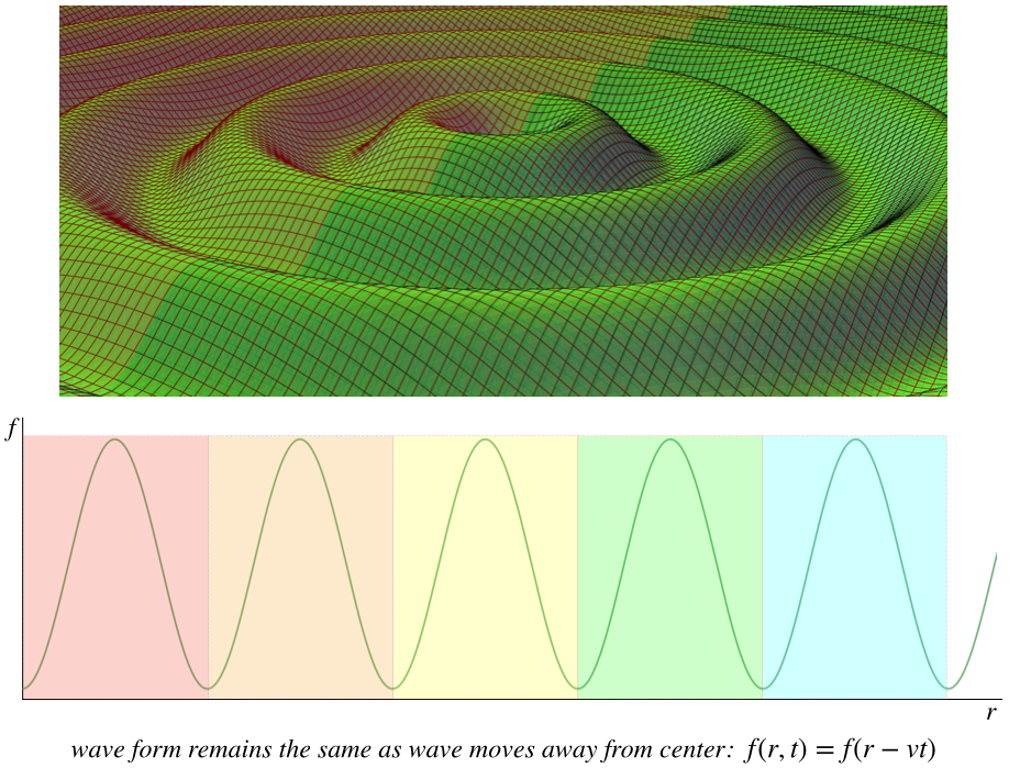
The graph shows a cross-sectional snapshot of the wave – the waveform repeats as a function of \(r\).

Figure 1.1.3 – Two-Dimensional Circularly-Radiating Function Satisfying 2-D Wave Equation

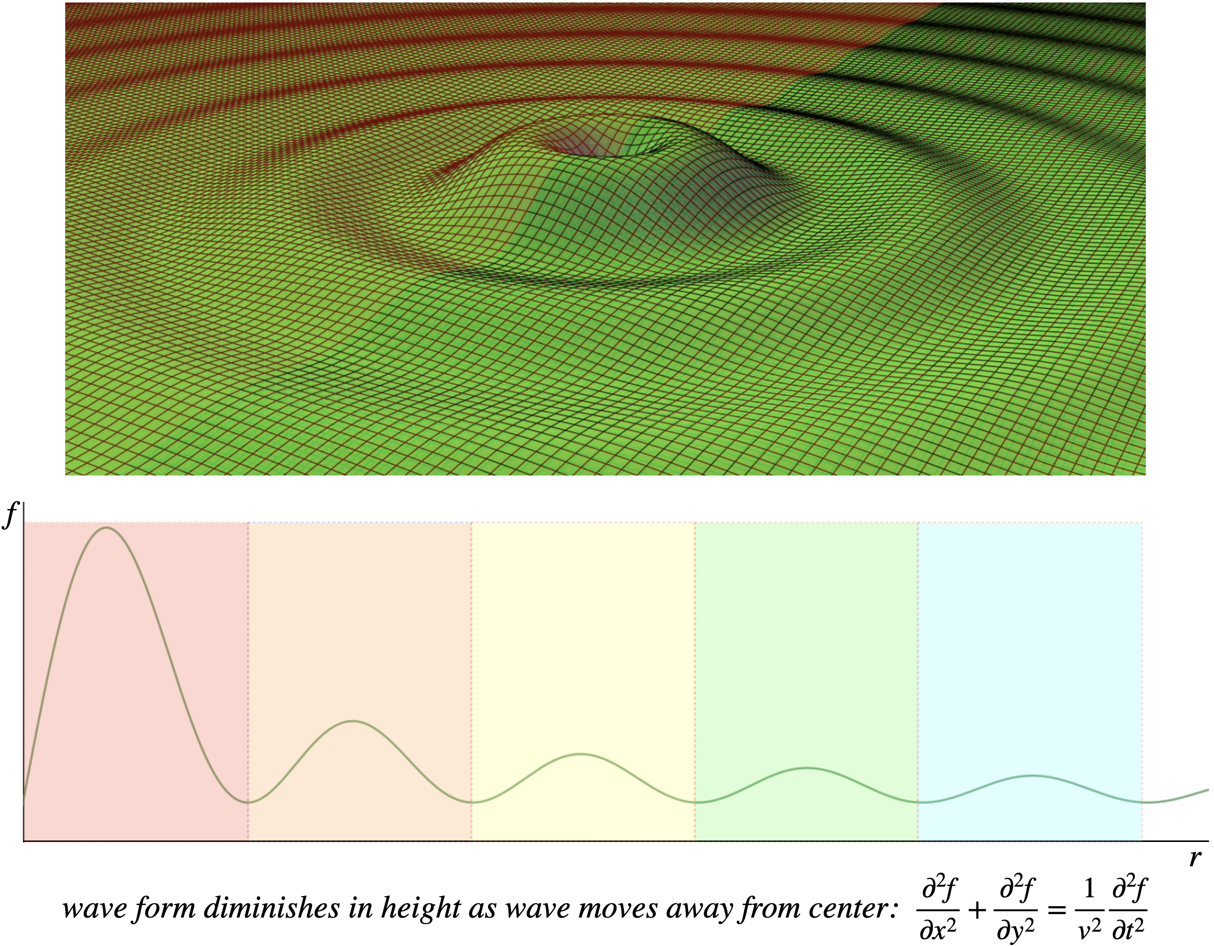
The graph shows a cross-sectional snapshot of the wave – the waveform does not repeat as a function of \(r\).

We can't answer this question purely mathematically – we have to observe what actually happens in nature. As we will see in Section 1.3, conservation of energy will require that it is in fact the extended two-dimensional wave equation that gives the correct answer – two and three-dimensional waveforms do not remain fixed as they radiate outward. The wave displacements diminish with distance from the source, as shown in Figure 1.1.3.

Finally, it should be mentioned that a shorthand notation is commonly used for the sum of the three-dimensional spatial double derivatives, which looks like:

\[\nabla^2 f = \dfrac{1}{v^2}\dfrac{\partial^2 f}{\partial t^2} \]

The differential equation given earlier is in cartesian coordinates \((x,y,z)\), but it could just as easily be written in cylindrical \((r,\theta,z)\) or spherical \((r,\theta,\phi)\) polar coordinates (though we won't do so here). This shorthand form avoids committing to a coordinate system altogether.