A2: Redshifts

[The 'A' series of chapters is an alternative start to the textbook in which chapters 1 through 4 are skipped, so that we dive right into an expanding spacetime.]

We introduced an expanding spacetime in the previous chapter. Now we begin to work out observational consequences of living in such a spacetime. In this and the next few chapters we will derive Hubble's Law, \(v=H_0 d\). In fact, we will derive a more general version of it valid for arbitrarily large distances.

Here we continue to work with just one spatial dimension. Assuming a homogeneous universe we have the same invariant distance rule as before:

\[ds^2 = -c^2 dt^2 + a^2(t)dx^2.\label{eqn:InvDistFRW1}\]

We derive in this chapter how the wavelength of light stretches over time, due to the expansion of the universe. This is called the cosmological redshift. We will find that the cosmological redshift is a very simple function of the scale factor at the time of emission divided by the scale factor at the time of reception. In other words, redshift tells us how much the universe expanded since light left the object we are observing.

In general, whether its origin is the expansion of space or the motion of an object, redshift is a quantification of the stretching of the wavelength of light. We use the symbol \(z\) to denote redshift and define it as:

\[z \equiv (\lambda_{\rm received} - \lambda_{\rm emitted})/\lambda_{\rm emitted}.\]

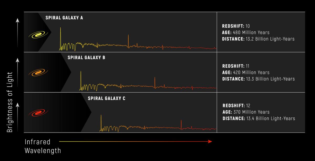
We see in the figure below (from NASA and Space Telescope Science Institute) some model spectra of galaxies with redshifts of 10, 11, and 12. One can see in the image that the same spectral features appear at longer wavelengths as the redshift increases. These features all had the same wavelength when emitted, but those wavelengths get stretched by the expansion to longer wavelengths. The further away the objects, the greater the stretching that occurs. We will explore this relationship between distance and redshift in chapter TBD. 

Next we want to derive the relationship between redshift and expansion for light that leaves an object at rest at time \(t_e\) and is observed today by an observer at rest at time \(t_r\). To help us get there we will first introduce what we call "conformal time" and then discuss the value of the invariant distance on paths traveled by light.

Note

By "at rest" we mean at rest in the coordinate system that has an invariant distance of the form in Equation \ref{eqn:InvDistFRW1}. This frame is called "cosmic rest." Note that for a frame that is moving with respect to cosmic rest, slices of constant time would be different, and we'd no longer have this simple form where the scale factor only depends on the time coordinate.

Conformal Time

You will recall from the previous chapter that in an expanding spacetime, light does not travel on straight lines. For calculational purposes, as we will see, it would be nicer if it did move on straight lines. Well, with a change of coordinates, it can! For this purpose, we introduce a coordinate called "conformal time." The conformal time, \(\eta\), is defined via \(d\eta = dt/a(t)\). In a conformal time diagram, for the expanding spacetime with which we have been working, light trajectories are straight lines. We will find that this is a very useful property.

Box \(\PageIndex{1}\)

Exercise 2.1.1: Given a spacetime described by Equation \ref{eqn:InvDistFRW1}, work out the invariant distance specified for \(\eta,x\) labeling instead of \(t,x\) labeling. You should find \( ds^2 = a^2(\eta)[-c^2 d\eta^2 + dx^2] \) where by \(a(\eta)\) we just mean \(a(t(\eta))\). Note that \(a(\eta)\) is simply shorthand for \(a(t(\eta)\).

Beware: in previous versions of this textbook we used \(\tau\) for conformal time and it's possible that in some places we still have the old notation. I found that the use of \(\tau\) caused some confusion for students because they have seen that used before for proper time, and these are not the same thing.

The Invariant Distance for Light Trajectories

The invariant distance for a path taken by a photon is always zero. You know this is true in special relativity where \(ds^2 = -c^2 dt^2 + dx^2\). Light always travels at the speed of light, so we always have \(dx = \pm c dt\), which in turn ensures that \(ds^2 = -c^2 dt^2 + c^2 dt^2 = 0\). To see that this is true more generally, first note that for an observer at rest in a given coordinate system, and given our physical interpretation of the invariant distance, the equation for the invariant distance can always be written schematically in terms of the trajectory of a moving object as

\(ds^2\) = \(-c^2\)(infinitesimal time elapsed)\(^2\) + (infinitesimal spatial distance traversed)\(^2\)

where by "infinitesimal time elapsed" we mean as measured by a clock that is not moving in the given coordinate system and by "infinitesimal spatial distance traveled" we mean as measured by a ruler that is not moving in the given coordinate system. You can immediately see that this is true in two steps. First, consider a purely spatial separation (in the given coordinate system). The invariant distance rule then tells you that the invariant distance squared is the square of the distance between the two points as measured by a ruler at rest in that coordinate system. This verifies the second term on the right-hand side of the above equation. Second, consider a purely temporal separation. The invariant distance rule tells you that the square of the invariant distance divided by \(-c^2\) gives the square of the time elapsed on a clock moving between these two points. This verifies the first term on the right-hand side of the above equation.

You know that in the special theory of relativity that all observers see light moving at speed \(c\). A version of this is true in general relativity. We just have to be careful to state it more locally. In the general theory, any observer seeing light pass right by them (through their location), will see it traveling with speed \(c\). Since this is true for all observers, it is also true for an observer at rest in the given coordinate system, so they will see (infinitesimal spacial distance traversed) = \(c \times\) (infinitesimal time elapsed). Putting this together with the above schematic equation for \(ds^2\) we see that for a light trajectory, \(ds^2 = 0\). 

Box \(\PageIndex{2}\)

Exercise 2.2.1: Draw how light rays move on a plot of \(x\) vs. \(\eta\) assuming our homogeneous expanding spacetime with one spatial dimension. Start from \(ds^2=0\) to find the relationship between \(d\eta\) and \(dx\), then draw a trajectory consistent with that relationship.

 

The theoretical relationship between redshift and scale factor history

We are all set up now to show, through the next three exercises, how redshift is related to the expansion that occurs between the time of emission of the light \(t_{\rm e}\), and the time of reception of the light, \(t_{\rm r}\). We will find the following very simple relationship stating that the wavelength has been increased by exactly the same factor by which the scale factor has increased; i.e.,

\[1+z \equiv \lambda_{\rm r}/\lambda_{\rm e} = a(t_{\rm r})/a(t_{\rm e}).\]

Box \(\PageIndex{3}\)

Exercise 2.3.1: Show that if \(\Delta t_e\) is the time interval between emitted light pulses (as measured by a stationary observer located where the emission is happening) and if \(\Delta t_r\) is the time interval between reception of first pulse and second pulse (as measured by a stationary observer located where the reception is occurring) then \(\Delta t_r/\Delta t_e = a(t_r)/a(t_e)\). To do so, use conformal time defined by \(d\eta = dt/a(t)\) and draw the pulse trajectories on an \(x\) vs. \(\eta\) diagram. By stationary observer we mean one that is at a constant value of \(x\); i.e., is at rest in the cosmic rest frame. You can assume that \(\Delta t_r\) and \(\Delta t_e\) are very short time scales compared to the time scale over which \(a(t)\) changes appreciably. Practical applications of this result often have \(a(t)\) changing on billion-year time scales and the \(\Delta t\)s shorter than nanoseconds so this assumption is well justified!

Box \(\PageIndex{4}\)

Exercise 2.4.1: Imagine propagation of electromagnetic waves. Use the above result to show that the wavelength of the waves emitted at time \(t_r\) and observed at time \(t_e\) is stretched so that:

\[\begin{equation*}
\begin{aligned}
z \equiv (\lambda_{\rm received} - \lambda_{\rm emitted})/\lambda_{\rm emitted} = a(t_r)/a(t_e) - 1
\end{aligned}
\end{equation*}\]

Hint: think about what happens to the period of the wave first, and then go from that to wavelength using the fact that wavelength is proportional to period.

Box \(\PageIndex{5}\)

Exercise 2.5.1: The most distant object for which a redshift has been measured is called a gamma-ray burst and it has a redshift of \(z=8.2\). By what factor has the universe expanded since light left that object?

We have just worked out the amazing fact that if we can identify a spectral line and measure its wavelength, then we can directly determine how much the universe has expanded since light left the object. Rearranging the result from Exercise 2.2.1 a little we can express this amazing fact as an equation:

\[1+ z = \lambda_{r}/\lambda_{e} = a(t_r)/a(t_e). \]

Look again at the figure above and notice that the more distant the object, the higher the redshift. This is because the more distant the object, the more time it took light to get to us from the object, and therefore the smaller the scale factor was at the time the light left the object, \(t_e\).

Before closing this section, we remind the reader of how redshifts due to the Dopper effect are related to speed -- a result we will use later in deriving Hubble's Law. If a source is moving away from you at speed v and emitting pulses with period \(T\), then the second pulse has to travel a distance \(vT\) further to get to you than was the case for the first pulse. So it's arrival will be delayed by a time \(vT/c\). Thus the period for the arriving pulses is \(T(1+v/c)\). Since wavelength is proportional to period this means the wavelength is stretched by a factor of \(1+v/c\), which means, by definition of the redshift \(z\), that \(z = v/c\). Note that our derivation has ignored the effect of relativistic time dilation. If the source had period \(T\) at rest, then if it were moving with speed \(v\) with respect to us, in our frame the period would be stretched to \(\gamma T\) and so the complete expression for \(z\) from the Doppler effect is \(1+z = \gamma (1+v/c)\). But we are only interested in this expression for small \(v/c\), for which \(\gamma \sim 1.\)

Summary

1. In an expanding homogeneous and isotropic universe, the ratio between the wavelength of light emitted by an observer at cosmic rest, \(\lambda_e\) at time \(t_e\) and the wavelength as measured by an observer at cosmic rest \(\lambda_r\) at time \(t_r\) is given by \[1+z \equiv \lambda_r/\lambda_e = a(t_r)/a(t_e)\] where \(a(t)\) is the scale factor at time \(t\) and the above equation defines the redshift \(z\). We can think of this as the wavelength stretching with the expansion.
2. In a non-expanding universe, a source moving away from an observer with \(v/c \ll 1\) has its light redshifted (wavelength stretched) by \[\lambda_r/\lambda_e= 1+v/c\] which is the normal Doppler effect you have studied before. What this implies is that if we interpret a small redshift \(z\) caused by the expansion of space as due to an ordinary motion-induced Dopper effect we will set \(z=v/c\). We will use this relationship later in our derivation of Hubble's Law: \(v = H_0 d\). The next thing we need for Hubble's law is how to measure distances, and how those measurements depend on theoretical quantities.

Additional Resources

You can look at images and spectra of galaxies in the Sloan Digital Sky Survey here. The spectra include identification of emission and absorption lines (with the atoms or ions responsible for them) and measurements of the redshift. To find the spectra and images, look for the table and click on the Object ID.

Quasar absorption line systems have particularly interesting spectra. You can read about them here.