
3.3: Particle Model of Bond Energy
- Page ID
- 19134

\( \newcommand{\vecs}[1]{\overset { \scriptstyle \rightharpoonup} {\mathbf{#1}} } \)
\( \newcommand{\vecd}[1]{\overset{-\!-\!\rightharpoonup}{\vphantom{a}\smash {#1}}} \)
\( \newcommand{\dsum}{\displaystyle\sum\limits} \)
\( \newcommand{\dint}{\displaystyle\int\limits} \)
\( \newcommand{\dlim}{\displaystyle\lim\limits} \)
\( \newcommand{\id}{\mathrm{id}}\) \( \newcommand{\Span}{\mathrm{span}}\)
( \newcommand{\kernel}{\mathrm{null}\,}\) \( \newcommand{\range}{\mathrm{range}\,}\)
\( \newcommand{\RealPart}{\mathrm{Re}}\) \( \newcommand{\ImaginaryPart}{\mathrm{Im}}\)
\( \newcommand{\Argument}{\mathrm{Arg}}\) \( \newcommand{\norm}[1]{\| #1 \|}\)
\( \newcommand{\inner}[2]{\langle #1, #2 \rangle}\)
\( \newcommand{\Span}{\mathrm{span}}\)
\( \newcommand{\id}{\mathrm{id}}\)
\( \newcommand{\Span}{\mathrm{span}}\)
\( \newcommand{\kernel}{\mathrm{null}\,}\)
\( \newcommand{\range}{\mathrm{range}\,}\)
\( \newcommand{\RealPart}{\mathrm{Re}}\)
\( \newcommand{\ImaginaryPart}{\mathrm{Im}}\)
\( \newcommand{\Argument}{\mathrm{Arg}}\)
\( \newcommand{\norm}[1]{\| #1 \|}\)
\( \newcommand{\inner}[2]{\langle #1, #2 \rangle}\)
\( \newcommand{\Span}{\mathrm{span}}\) \( \newcommand{\AA}{\unicode[.8,0]{x212B}}\)
\( \newcommand{\vectorA}[1]{\vec{#1}} % arrow\)
\( \newcommand{\vectorAt}[1]{\vec{\text{#1}}} % arrow\)
\( \newcommand{\vectorB}[1]{\overset { \scriptstyle \rightharpoonup} {\mathbf{#1}} } \)
\( \newcommand{\vectorC}[1]{\textbf{#1}} \)
\( \newcommand{\vectorD}[1]{\overrightarrow{#1}} \)
\( \newcommand{\vectorDt}[1]{\overrightarrow{\text{#1}}} \)
\( \newcommand{\vectE}[1]{\overset{-\!-\!\rightharpoonup}{\vphantom{a}\smash{\mathbf {#1}}}} \)
\( \newcommand{\vecs}[1]{\overset { \scriptstyle \rightharpoonup} {\mathbf{#1}} } \)
\(\newcommand{\longvect}{\overrightarrow}\)
\( \newcommand{\vecd}[1]{\overset{-\!-\!\rightharpoonup}{\vphantom{a}\smash {#1}}} \)
\(\newcommand{\avec}{\mathbf a}\) \(\newcommand{\bvec}{\mathbf b}\) \(\newcommand{\cvec}{\mathbf c}\) \(\newcommand{\dvec}{\mathbf d}\) \(\newcommand{\dtil}{\widetilde{\mathbf d}}\) \(\newcommand{\evec}{\mathbf e}\) \(\newcommand{\fvec}{\mathbf f}\) \(\newcommand{\nvec}{\mathbf n}\) \(\newcommand{\pvec}{\mathbf p}\) \(\newcommand{\qvec}{\mathbf q}\) \(\newcommand{\svec}{\mathbf s}\) \(\newcommand{\tvec}{\mathbf t}\) \(\newcommand{\uvec}{\mathbf u}\) \(\newcommand{\vvec}{\mathbf v}\) \(\newcommand{\wvec}{\mathbf w}\) \(\newcommand{\xvec}{\mathbf x}\) \(\newcommand{\yvec}{\mathbf y}\) \(\newcommand{\zvec}{\mathbf z}\) \(\newcommand{\rvec}{\mathbf r}\) \(\newcommand{\mvec}{\mathbf m}\) \(\newcommand{\zerovec}{\mathbf 0}\) \(\newcommand{\onevec}{\mathbf 1}\) \(\newcommand{\real}{\mathbb R}\) \(\newcommand{\twovec}[2]{\left[\begin{array}{r}#1 \\ #2 \end{array}\right]}\) \(\newcommand{\ctwovec}[2]{\left[\begin{array}{c}#1 \\ #2 \end{array}\right]}\) \(\newcommand{\threevec}[3]{\left[\begin{array}{r}#1 \\ #2 \\ #3 \end{array}\right]}\) \(\newcommand{\cthreevec}[3]{\left[\begin{array}{c}#1 \\ #2 \\ #3 \end{array}\right]}\) \(\newcommand{\fourvec}[4]{\left[\begin{array}{r}#1 \\ #2 \\ #3 \\ #4 \end{array}\right]}\) \(\newcommand{\cfourvec}[4]{\left[\begin{array}{c}#1 \\ #2 \\ #3 \\ #4 \end{array}\right]}\) \(\newcommand{\fivevec}[5]{\left[\begin{array}{r}#1 \\ #2 \\ #3 \\ #4 \\ #5 \\ \end{array}\right]}\) \(\newcommand{\cfivevec}[5]{\left[\begin{array}{c}#1 \\ #2 \\ #3 \\ #4 \\ #5 \\ \end{array}\right]}\) \(\newcommand{\mattwo}[4]{\left[\begin{array}{rr}#1 \amp #2 \\ #3 \amp #4 \\ \end{array}\right]}\) \(\newcommand{\laspan}[1]{\text{Span}\{#1\}}\) \(\newcommand{\bcal}{\cal B}\) \(\newcommand{\ccal}{\cal C}\) \(\newcommand{\scal}{\cal S}\) \(\newcommand{\wcal}{\cal W}\) \(\newcommand{\ecal}{\cal E}\) \(\newcommand{\coords}[2]{\left\{#1\right\}_{#2}}\) \(\newcommand{\gray}[1]{\color{gray}{#1}}\) \(\newcommand{\lgray}[1]{\color{lightgray}{#1}}\) \(\newcommand{\rank}{\operatorname{rank}}\) \(\newcommand{\row}{\text{Row}}\) \(\newcommand{\col}{\text{Col}}\) \(\renewcommand{\row}{\text{Row}}\) \(\newcommand{\nul}{\text{Nul}}\) \(\newcommand{\var}{\text{Var}}\) \(\newcommand{\corr}{\text{corr}}\) \(\newcommand{\len}[1]{\left|#1\right|}\) \(\newcommand{\bbar}{\overline{\bvec}}\) \(\newcommand{\bhat}{\widehat{\bvec}}\) \(\newcommand{\bperp}{\bvec^\perp}\) \(\newcommand{\xhat}{\widehat{\xvec}}\) \(\newcommand{\vhat}{\widehat{\vvec}}\) \(\newcommand{\uhat}{\widehat{\uvec}}\) \(\newcommand{\what}{\widehat{\wvec}}\) \(\newcommand{\Sighat}{\widehat{\Sigma}}\) \(\newcommand{\lt}{<}\) \(\newcommand{\gt}{>}\) \(\newcommand{\amp}{&}\) \(\definecolor{fillinmathshade}{gray}{0.9}\)Overview
In this section we develop the Particle Model of Bond Energy. We start with the idea of adding enough energy to break a bond between two subatomic particles interacting with a Lennard-Jones potential. We then proceed to thinking about how much energy is needed to break bonds between multiple particles. At the end of this section, we come up with an approximation that will allow us to easily estimate the bond energy of a macroscopic substance and compare to experimentally determined values of enthalpy we saw in Chapter 1.
Microscopic Bond Energy
In the previous section we modeled two neutrally interacting atoms or molecules with a pair-wise Lennard-Jones potential. Since this potential energy closely mimics the behavior of the spring-mass system (at least near equilibrium), we can think of two interacting particles as being connected by a spring as shown in the figure below. Unlike a "standard" spring, the spring connecting two particles gets very stiff when the particles are very close together (the slope of PELJ is very steep for \(r<r_o\)), weak as particles move apart (slope decreases for \(r>r_o\), until the spring "breaks apart" for larger separations of \(r\gtrsim 3r_o\). The figure also shows the equilibrium separation, \(r_o\), between two such atoms. Since \(r_o=1.12\sigma\) the two atoms are nearly touching as pictured. (Recall, we measure particle separation using center-to-center distances, so two touching atoms would have a separation of \(\sigma\)).
Figure 3.4.1: Two interacting neutral atoms.

To calculate the energy required to break a bond, let us assume that the two atoms are motionless at equilibrium separation of \(r_o\). The initial total energy of these atoms is then \(E_{\text{tot,initial}}=PE(r_o)=-\varepsilon\). We discussed in the previous section that as long as \(E_{tot}\) is less than zero the particles remain bound. When \(E_{tot}\) becomes greater than zero the two particles become unbound and are very far apart, \(r\gg r_o\). If we assume that the atoms remain motionless (KE=0) after enough energy is added to break the bond, the total final energy will be zero since at large separations \(PE_{LJ}(r\gg r_o)\sim 0\). The amount of energy required to break the bond between two atoms that are initially at equilibrium is:
\[\Delta E=E_f-E_i=0-(-\varepsilon)=\varepsilon\]
We can think of this quantity as the change of bond energy of the two particle system initially at equilibrium. As we discussed in Chapter 1 energy is required to break bonds, thus the change in bond energy has to be positive when a bonds are broken, such as for a phase transition from liquid to gas. We see the same result here on a microscopic scale.
Since we want to transition to a macroscopic scale, let us start adding atoms to our physical system. Below is a illustration of three atoms, all at equilibrium separations.
Figure 3.4.2: Three interacting neutral atoms.
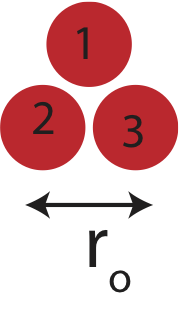
If we want to know the energy required to break up the three atom structure, we need to consider the three bonds present: 1-2, 1-3, and 2-3. Since, all three pairs are separated by \(r_o\), the initial energy of these motionless atoms is simply the sum of the potential energies of the three pairs:
\[E_{\text{tot,initial}}=PE_{12}(r_o)+PE_{13}(r_o)+PE_{23}(r_o)=-3\varepsilon\]
As before, the energy of the system when all three atoms are unbound or at far separations is zero, \(E_{\text{total,final}}=0\), so the energy required to break this structure is \(\Delta E=+3\varepsilon\).
For now, we will stick to two-dimensional structures for simplicity. Let us consider a structure of four atoms keeping them as close as possible to each other, as shown below.
Figure 3.4.3: Four interacting neutral atoms.
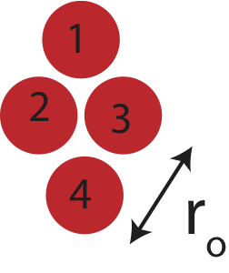
As before we need to break all the bonds present for this structure to become unbound. For the four atom structure there are 6 bonds: 1-2, 1-3, 1-4, 2-3, 2-4, and 3-4. However, it is no longer possible to arrange four atoms in two-dimensions so all of them are at the \(r_o\) separation. From the figure above we can see that atoms 1 and 4 are not separated by \(r_o\). We can use Pythagorean theorem to find the distance between atoms 1 and 4:
\[r_{14}=2\sqrt{(r_o)^2-\Big(\frac{r_o}{2}\Big)^2}=\sqrt{3}r_o\]
See Figure 3.4.4 below for the geometry of calculating this distance. We call atoms that are separated by the shortest possible distance, nearest neighbors, sometimes abbreviated as nn. The pairs that have the next possible shortest distance in a given configuration are known as the next-to-nearest neighbors, sometimes abbreviated as nnn. In the four-atom example pairs 1-2, 1-3, 2-3, 2-4, and 3-4 are nearest neighbors, and pair 1-4 are next-to-nearest neighbors.
As for the three-atom case, the initial total energy is the sum of all the pair-wise potential energies. Except for the four-atom system, there is now one pair whose potential energy is no longer evaluated at \(r_o\), but rather at \(\sqrt{3}r_o\). To break the 1-4 bond will require less energy since its initial energy is no longer the minimum potential energy of \(-\varepsilon\). Figure 3.4.4 graphically illustrates the value of \(PE_{LJ}(\sqrt{3}r_o)\). Since the x-axis is in units of \(\sigma\), the separation needs to be converted to these units. Using \(r_o=1.12\sigma\), the separation between atoms 1 and 4 is \(r=\sqrt{3}r_o=1.94\sigma\) as marked on the plot. If we read the value directly from the plot we get \(PE_{LJ}(\sqrt{3}r_o)\sim -0.07\varepsilon\). A more accurate method would be to plug in this separation into the Lennard-Jones Equation 3.2.1 directly:
\[PE_{LJ}(r=1.94\sigma)=4\varepsilon\Big [\Big(\frac{\sigma}{1.94\sigma}\Big)^{12}-\Big(\frac{\sigma}{1.94\sigma}\Big)^6 \Big]=-0.074\varepsilon \]
Figure 3.4.4: Finding equilibrium energy for a four-atom structure.

The initial total energy of the four-atom two-dimensional system is given by:
\[E_{\text{tot,initial}}=PE_{12}(r_o)+PE_{13}(r_o)+PE_{23}(r_o)+PE_{24}(r_o)+PE_{34}(r_o)+PE_{14}(\sqrt{3}r_o)=-5\varepsilon-0.074\varepsilon\simeq -5.07\varepsilon\]
The three systems we analyzed so far in 2D (two-atom, three-atom, and four-atom) are all still considered microscopic since they consist only of a few atoms. Next, we want to see how to extend this analysis for a macroscopic (on the order of one mole, \(\sim 10^{23}\) number of particles) system.
Macroscopic Bond Energy
As we continue to add atoms to our two-dimensional structure we come up with the following picture:
Figure 3.4.5: Macroscopic 2D atom structure.
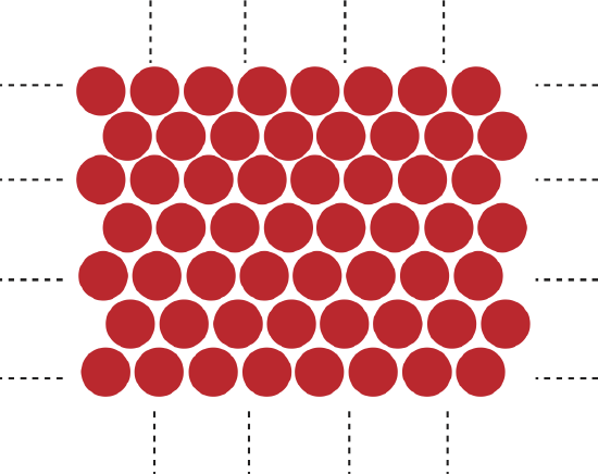
The dashed lines indicate that the atoms continue indefinitely. In order to calculate the amount of energy required to break up this structure we would need to consider all the pairs that are present in this structure. We saw when calculating the energy required to break just a few atoms, we set the initial energy of the structure when all atoms are motionless at equilibrium. When we added enough energy to break up all the bonds in a structure, while keeping the kinetic energy of the particles zero, we found that the final energy was always zero, since the pair-wise potential energy goes to zero when the particles are far apart.
Since the system is now macroscopic we can start drawing connections between the pair-wise potential that binds microscopic particles together to the change of bond energy we discussed in Chapter 1 during a phase transition for a macroscopic pure substance. We can write the change in bond energy as:
\[\Delta E_{bond}=E_{bond,final}-E_{bond,initial}\]
Comparing the above equation to our analysis of microscopic structure we see that \(E_{bond,initial}\) (such as the bond energy of a solid or liquid) corresponds to \(E_{total,initial}\), while \(E_{bond,final}\) (bond energy of a gas where particles are no longer interacting) is \(E_{total,final}\) which is zero. We define the bond energy in the Particle Model of Bond Energy of a substance as the sum of all of the pair-wise potential energies of the particles comprising the substance, calculated when all of the particles are at their equilibrium positions corresponding to a particular physical and chemical state:
\[ E_{bond} = \sum_{all-pairs}PE_{LJ} \text{(evaluated at equilibrium separations)}\label{pair.bond}\]
In solid and liquid phases there is a bond energy associated with the attractive part of all the pair-wise potential energies acting between pairs of particles. Energy must be added to separate the particles sufficiently far apart, thus breaking the bonds. Since the maximum value of the bond energy occurs when the particles are widely separated, and because of the way the pair-wise potential is defined, the bond energy of liquids and solids must be less than zero; that is, the bond energy is negative. Energy required to break the bonds or the change in bond energy is simply the magnitude of the bond energy and is always a positive number, even though the bond energy is negative.
Alert
By convention, all pair-wise potentials are defined to be zero when the particles are separated sufficiently so that the force acting between the particles is zero and negative when the particles are bound. Therefore, the bond energy of any condensed substance (solid of liquid) is always negative. The maximum value of the bond energy is zero when the particles that comprised the substance are all completely separated to large distances. This is sometimes hard to get our minds around. But it simply has to do with our choice of where to set the zero potential energy as we discussed in the previous section as well as in our discussion of setting the origin for the gravitational potential energy. What matters is that that the change in bond energy when bonds are broken is positive, which is the case here since we start with a negative bond energy and end up with zero bond energy.
If we attempt to calculated the bond energy as defined in Equation \ref{pair.bond} for the 2D structure in Figure 3.4.5, we can see that very quickly that this calculation becomes extremely overwhelming due to the number of pairs involved. It is certainly not possible to do without a computer. Before relying on computers to do our work, physicists often prefer to understand nature by simplifying things, even if it means making some assumptions, as long as they are reasonable. We saw for a four-atom system that the energy required to break next-to-nearest neighbor pair was \(0.07\varepsilon\), which significantly less then the energy of \(\varepsilon\) required to break a nearest neighbor pair.
Thus, let us approximate the bond energy Equation \ref{pair.bond} by only considering nearest neighbor pairs separated by \(r_o\). Since the value of the pair-wise potential for a nearest neighbor pair is the potential minimum, \(PE_{LJ}(r_o)=-\varepsilon\), this approximation results in:
\[E_{bond} \approx – (\text{total number of nn pairs}) \times\varepsilon\label{Ebond.app}\]
If we revisit to our 2D structure in Figure 3.4.5 we can easily apply this approximation without having to reply on a computer. The only task is to calculate the total number of nearest neighbors. If we focus on some central atom in the figure, we count that it has 6 nearest neighbors. This is true for any atom in the structure, except for the ones at the very edge. However, we we want to focus on one mole, \(N_A=6.02\times 10^{23}\), of atoms, so the majority of atoms will not be at the edge. Thus, we will neglect edge effects. You might be tempted to say the the total number of nearest neighbors (neglecting edge effects) is just 6 times the number of atoms. To see why this is not correct, let us return to the three atoms in Figure 3.4.2. Of course, here we can just count the pairs directly (there are three!), but if we applied the described method we would say that each atom has 2 neighbors, there are 3 atoms, thus 6 neighbors. This is double of the actual number of bonds! Thus, taking double counting into account, the total number of nearest-neighbor pairs, Nnn, for a general structure of N atoms:
\[N_{\text{nn}}=\frac{N}{2}\times (\text{# nn per atom})\label{number.nn}\]
In the real world, at least more common everyday substances that we analyzed in Chapter 1, such as water, lead, and gold, are three-dimensional in nature. The number of neighboring atoms and their distances will depend on a particular structure that a substance form when in the solid phase. An example of a common one, known a the face-centered cubic (fcc) structure has 12 nearest neighbors as shown in the figure below.
Figure 3.4.6: Nearest neighbors of a 3D fcc structure.
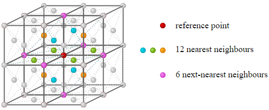
Applying Equations \ref{Ebond.app} and \ref{number.nn} for one mole of a "standard" solid, the bond energy is:
\[E_{bond} \approx – 6N_A\times\varepsilon\]
Do we need to worry about interactions between atoms or molecules that are not nearest neighbors? A little bit, depending on how accurate we want our numerical predictions to be. Looking back at the pair-wise potential energy curve, we see that the slope is not fully horizontal when the particles are located two diameters from each other. There are a lot of nearby neighbors that are within two diameters of each other, so these non-nearest neighbors will still be attracting each other a little bit and will make a contribution to the bond energy, but typically significantly less than the nearest neighbors. This approximation, however, will tend to underestimate the bond energy. The underestimation comes in because we have not added in the contributions of the many neighbor pairs that are in the one to two diameter separation range.
This definition of bond energy avoids the issue of the thermal energy possibly changing, because the calculation is carried out at essentially zero Kelvin (all particles are in their equilibrium positions as they would be at absolute zero, if the phase actually existed at absolute zero) in both the bound state as well as when the particles are separated. We take this to be our technical definition of bond energy. An equivalent definition would be to say that the energy required to separate the particles is carried out so that the thermal energy is the same after the separation as before the separation. We will incorporate thermal energy into our model in the next section.
The empirically determined heats of melting and heats of vaporization are reasonable approximations to the changes in bond energy at the respective physical phase changes. There are a few tricky aspects associated with directly relating bond energies to heats involved in phase changes. We will see our Particle Model of Thermal Energy that there are changes in the thermal energy at a phase change as well as in the bond energy. The empirically determined ∆H’s that we used in the bond energy system in Chapter 1, however, do incorporate any changes of energy in thermal energy at a phase change. Thus, the ∆H’s are not precisely a measure of the particle model bond energy change. For the most part we will ignore this until we have sufficient background to make sense of it. There are also several other rather subtle effects that we will ignore until we are ready to make sense of them in Chapter 4. We have also assume that the structure goes from a solid phase (all particles at equilibrium) to a gas phase (all particles unbound), completely ignoring what happens during the solid to liquid phase transition. For now we will make the approximation that connects the microscopic and the macroscopic definitions of bond energy:
\[\Delta E_{bond}\approx |\Delta m\Delta H|\]
Example \(\PageIndex{1}\)
UC Davis scientists continue to conduct experiment on the two new atoms, Aggieum (Ai) and Cyclerium (Cy). The plot below shows Lennard-Jones potential energies for Ai-Ai and Cy-Cy atoms.

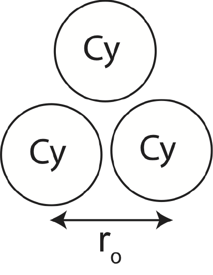
a) Calculate Ebond for the configuration shown below. Include all pair-wise interactions.
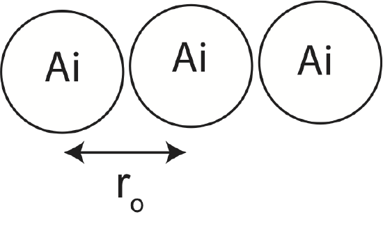
b) Calculate Ebond for another configuration shown below. Include all pair-wise interactions.
c) If the configuration in b) was instead a linear chain of 1 mole of Ai atoms, calculate the bond energy including only nearest-neighbor interactions. Include the effect of atoms at the edges. Do edge effects make a significant contribution to bond energy?
- Solution
-
a) There are 3 nearest neighbor bonds. For Cy, \(PE(r_o)=-0.6\times 10^{-21} J\). Therefore:
\[E_{bond}=-3\times PE(r_o)=3\times(-0.6\times 10^{-21})=-1.8\times 10^{-21}J\]
b) There are 2 nearest neighbor bonds. For Ai, \(PE(r_o)=-1.0\times 10^{-21}J\). There is also one next-to-nearest neighbor bond at:
\[r=2r_o=2\times 1.12\sigma=2.24\sigma=2.24\times 10^{-10}m\]
It is possible to read \(PE(r=2.24\times 10^{-10}m)\) from the plot, but it is more accurate to plug this values into the Lennard-Jones equation:
\[PE_{LJ}(r=2.24\sigma)=4\varepsilon\Big [\Big(\frac{\sigma}{2.24\sigma}\Big)^{12}-\Big(\frac{\sigma}{2.24\sigma}\Big)^6 \Big]=-0.031\varepsilon \]
Thus:
\[E_{bond}=-2\times (1\times 10^{-21}J)-0.031\times 10^{-21} J=-2.031\times 10^{-21}J\]
c) Each atom has 2 nearest neighbors in a linear chain. The total number of nn for one mole is \(\frac{N_A}{2}\times 2=N_A\). However, there are two extra bonds we are counting at the two edges. But the edges are not double counted, so we need to subtract one bond. If we account for this, \(N_{nn}=N_A-1\) and the bond energy becomes:
\[E_{bond}\approx -(1\times 10^{-21}J)\times(N_A-1)=-602J\]
Since \(N_A\gg 1\), edge effect are truly negligible, which is typically the case for a macroscopic structure.