
8.1: Graphing Motion


- Last updated
- Nov 8, 2022
- Save as PDF

( \newcommand{\kernel}{\mathrm{null}\,}\)
Force and Kinematics
Our focus so far has been on the details of force, and comparing the motion of an object before and after the force acted on the object, typically at two time instances. We will now look at the motion of an object for a continuous duration of time while a net force acts on the system or when the net force is zero. We first do this by graphically representing the time dependence of motion by analyzing acceleration, velocity, and position as a function of time. These three vectors are connected by the following equations that we have introduced in the earlier chapters:
→v=d→xdt; →a=d→vdt
We will see how to make sense of these equations graphically by looking at a few specific examples. Below are plots demonstrating motion of a box which is initially moving to the right with a net force also pointing to the right.
Figure 8.1.1: Force and Initial Velocity in the Same Direction
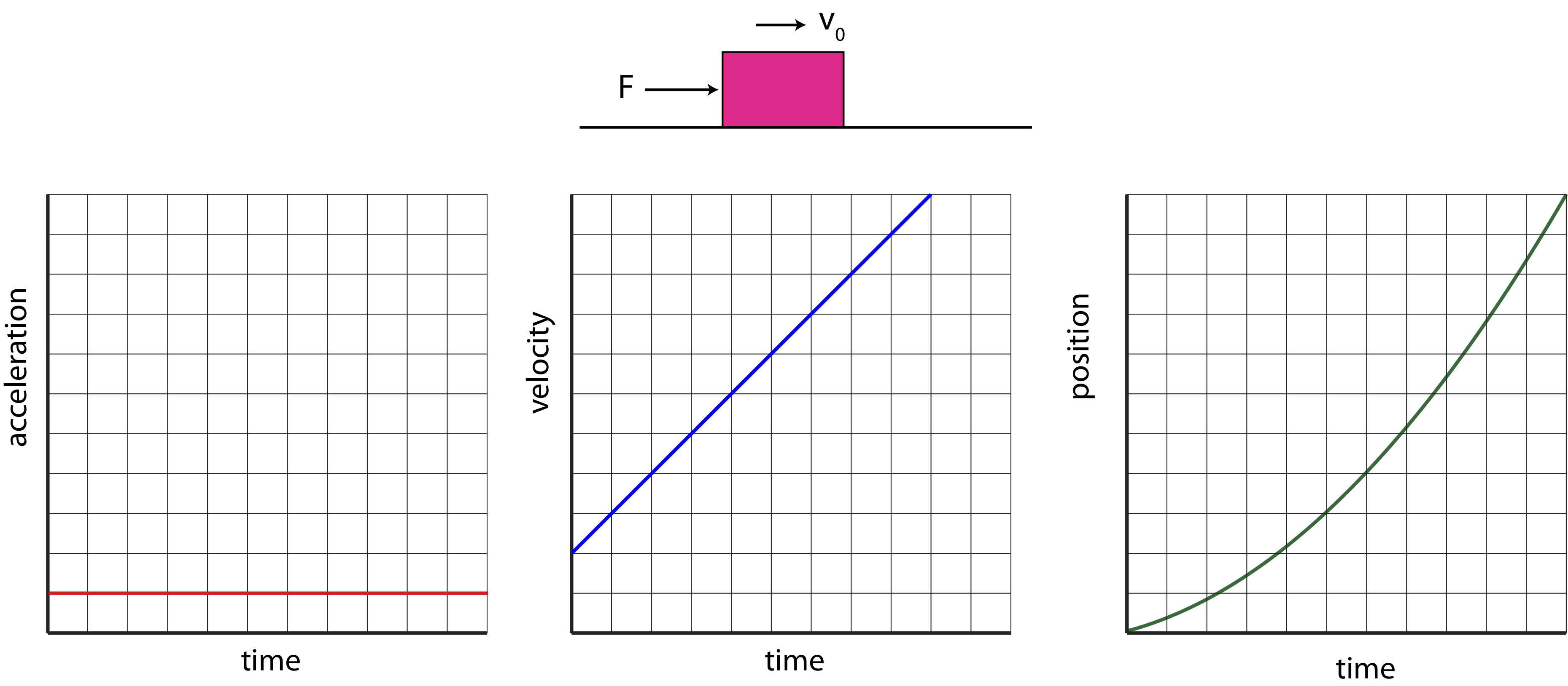
By convention we define to the right as positive. Then, acceleration will be positive as well according to Newton's second law since the net force is pointing to the right. We assume that the force is constant over this time range, resulting in acceleration being constant as well. Thus, acceleration plotted as a function of time is a horizontal line, as shown in Figure 8.1.1. The acceleration is arbitrarily chosen as 1 grid unit on this scale.
Equation ??? states that the slope of the velocity plot will give acceleration. This means that if acceleration is a constant, velocity must be linear as a function of time with a slope of 1 unit. This is consistent with Newton's second law which states that when there is a net force acting on the system, acceleration is non-zero, which implies that velocity is changing. There are infinite ways to have velocity changing with time with a slope of 1, since the line can intersect anywhere on the y-axis and have the same slope. Thus, another piece of information that is required to make the velocity versus time plot is the initial velocity at t=0. In the example in Figure 8.1.1 the initial velocity, vo, is arbitrarily set to 2 units. From the velocity plot we can see that the box is speeding up, since its speed is increasing with time.
Lastly, Equation ??? states that the slope of position plot is the velocity plot. In this case since velocity is linear and increasing, this means that the slope of position plot increases with time, and it does so in a quadratic manner. Thus, the position versus time plot in Figure 8.1.1 has a parabolic shape. As for the velocity plot, there are infinite ways to have the have shape, since the plot can be moved vertically up or down while retaining its slope. So we need to define the origin in order to determine where the position crosses the y-axis. It is convenient to define that origin at initial time, so in this case the position is zero at t=0. The position versus time tells us that the object is moving to the right and speeding up since the slope is positive and increasing with time.
Let us now turn to another example where the force and the initial velocity point in opposite direction as shown in Figure 8.1.2 below. The box is still moving to the right initially, but the force now points to the left. We will again assume that the force is constant over the time range that we want to analyze the motion of the box.
Figure 8.1.2: Force and Initial Velocity in the Opposite Directions
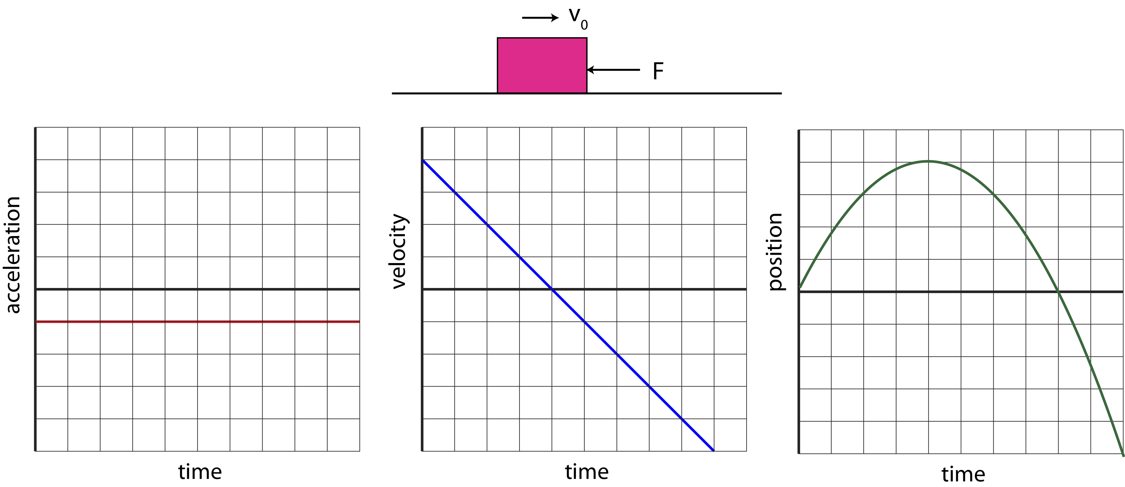
In this example acceleration is negative since the net force is to the left. Again, we choose a magnitude of 1 unit on this scale to represent constant acceleration over this time range. This means that velocity will have a slope of negative 1 units. Again, we need to choose initial velocity, and in this case we choose 4 units as shown in Figure 8.1.2. The initial velocity is positive since the box is moving to the right, but we see from the plot that when the slope is negative, the velocity plot will cross the x-axis and will start increasing in the negative direction. This means that initially the box is slowing down as the magnitude of velocity decreases, since the force is in the opposite direction of position. But at the moment when the velocity plot crosses the x-axis (at 4 units of time), the box temporarily stops, after which it turns around and starts moving in the negative direction. Recall, since velocity is a vector, negative velocity means that its it moving in the negative direction. And since the velocity is getting more negative after the box turns around, the speed, which is the magnitude of velocity, is increasing, so the box is now speeding up. The box starts to speed up after 4 units of time, the motion of the box is now in the same direction as the force.
For the position plot, we set the origin at the initial time again as seen in Figure 8.1.2. The shape of the plot is again parabolic since its slope has to be linear based of the velocity plot. Initially, the slope is positive and decreasing, corresponding to the box moving to the right and slowing down. At time of 4 units the slope of the position plot is zero. This is the exact time when the velocity goes to zero before the box turns around. After this, the slope of the parabolic shape negative and increasing since the box is now moving to the left and speeding up. Note, that the position is not negative when the box starts moving to the left, since negative position just means that the box is to the left of the origin. Initially, the box moved to the right of the origin, as it was slowing down. When it first turned around and started moving to the left, it was still to the right of the origin until it returned back to its starting position, exactly at 8 units of time on the position plot. After this, the box is located to the left of the origin, thus, position is negative.
As you work with analysis of motion for different physical situations, here are a list of a few key points to keep in mind when making acceleration, velocity and position plots:
General:
- Acceleration, velocity, and position are vectors which can have positive, negative, or zero values depending on their direction and location of origin.
- If you know one of the graphs, you can obtain the other two as long as you know initial conditions.
Acceleration:
- Acceleration points in the same direction as the net force.
- Acceleration is zero when the net force is zero.
- Acceleration plot alone does not contain any information whether the object is speeding up or slowing down, since it does not tell you which way the object is moving, only in which direction its velocity is changing.
Velocity:
- The slope of the velocity plot is the acceleration.
- Initial velocity has to be known to make the velocity versus time plot.
- When acceleration and velocity have the same sign, the system is speeding up.
- When acceleration and velocity have opposite signs, the system is slowing down.
- When velocity plot crosses the x-axis (changes sign), the system is turning around.
- When the slope of velocity plot is zero, acceleration is zero, implying zero net force.
Position:
- The slope of the position plot is the velocity.
- Initial position has to be known to make the position versus time plot.
- Positive slope means the object is moving to the right.
- Negative slope means the object is moving to the left.
- Increasing magnitude of slope (either negative or positive) means the object is speeding up.
- Decreasing magnitude of slope (either negative or positive) means the object is slowing down.
- Zero slope means the object is stationary.
- When the sign of the slope of the position plot changes, this means the object has changed direction of motion.
- The sign of the position plot does not tell us about the direction of motion, but an indication of whether the object is located on the positive or negative side of the origin.
Example 8.1.1
Below is a velocity versus time plot.
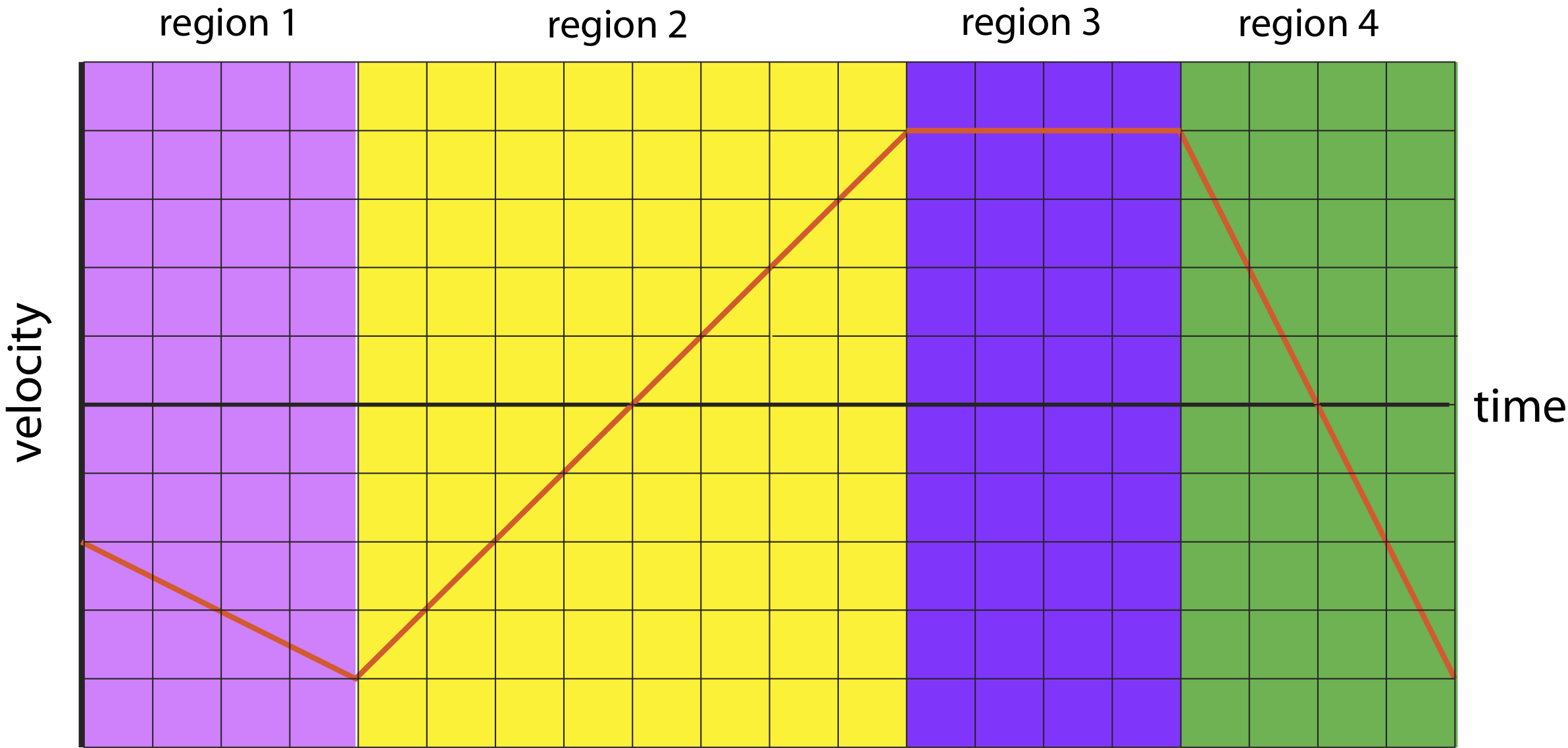
a) For each marked region specify the direction of motion (right, left, or turning around) and describe the speed (zero, speeding up, slowing down, or constant speed).
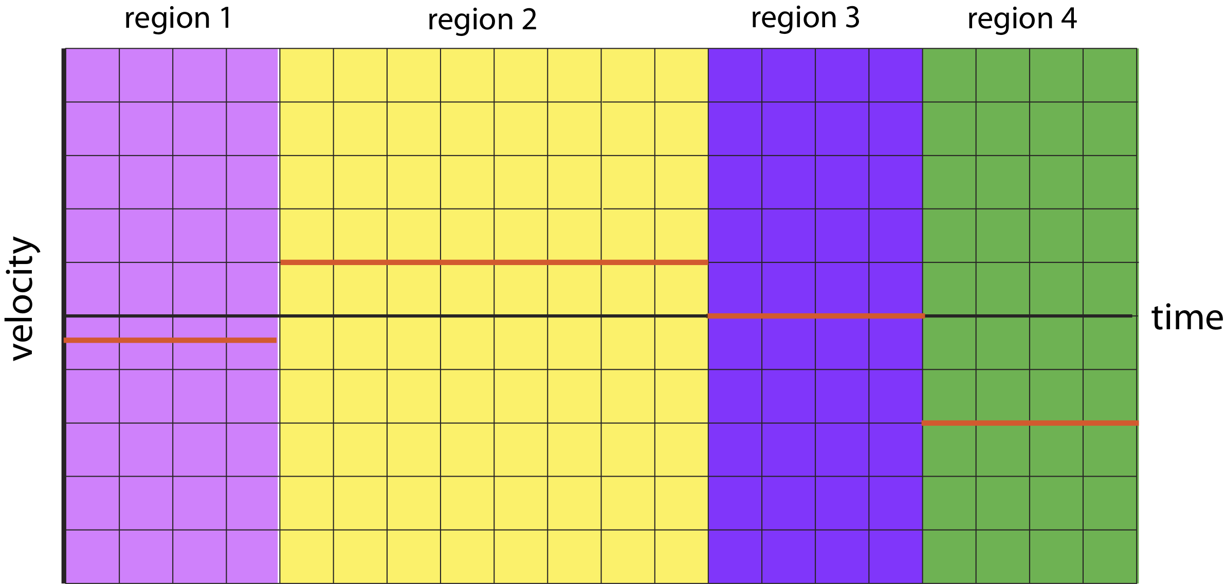
b) Make an acceleration versus time plot for the entire time shown.
- Solution
-
a) Region 1: object starts with non-zero velocity, is moving to the left since velocity is negative and speeding up since the magnitude of velocity is increasing.
Region 2: object is moving to the left and slowing down. After 4 units of time in this region, the object turns around, after which it's moving to the right and speeding up.
Region 3: object is moving to the right with constant speed.
Region 4: object is moving to the right and slowing down, after 2 units of time it turns around, then moving to the left and speeds up.
b) Below is the acceleration versus time plot. The plots in each region are obtained from the slope of velocity versus time plot for each marked region: region 1 the slope is -1/2, in region 2 the slope is 1, in region 3 the slope is zero, and in region 4 the slope is-2.
Example 8.1.2
Shown below is a rollercoaster ride. At the start of a drop, defined as t=0 sec, the train is moving with a speed of 6 m/s. The rest of the motion is depicted in the picture below. Assume the track is frictionless from t=0 to t=20sec. Between t=20sec and 30sec, the breaks create friction with the tracks. For this problem assume that the x-axis always points horizontal to the track (in the direction of motion), and the y-axis points perpendicular to the track, as depicted in the picture.
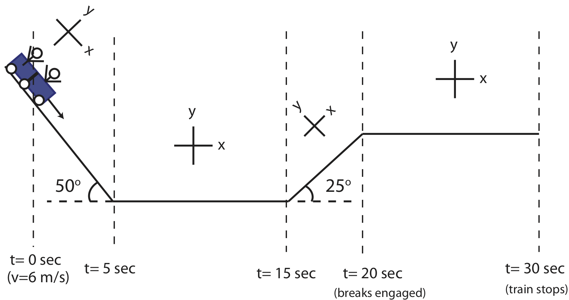
a) Draw four force diagrams for the train at t=2 sec, t=12 sec, t=18 sec, and t=25 sec. For each force diagram, split the forces into x-components (horizontal to the track) and y-component (perpendicular to the track).
b) Make a plot for component of velocity and acceleration horizontal the track (x-direction as shown in the figure) as a function of time from t=0 to t=30 sec.
- Solution
-
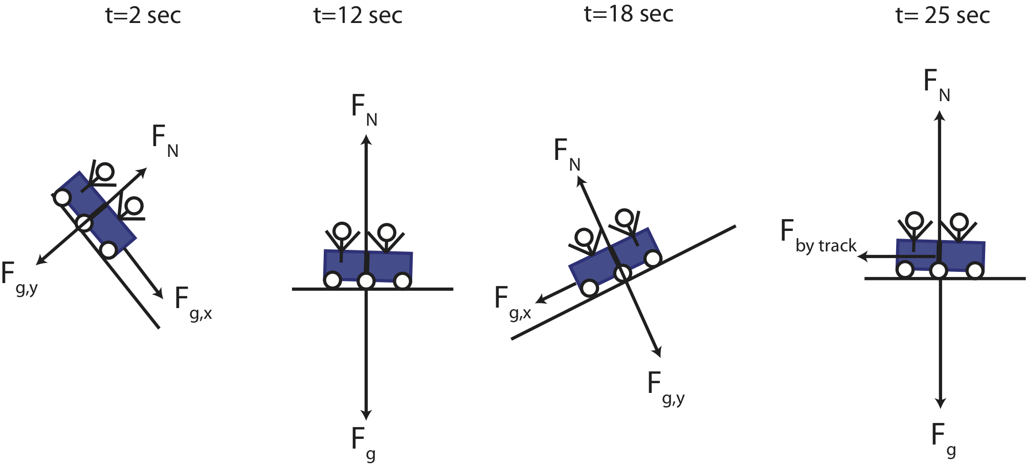
a) The free-body diagrams are shown below.
t=2 sec: in the first 5 seconds the track is frictionless, so there is only the force of gravity and the normal force. Gravity always points down, so it has a component along the track (x-direction in the tilted axis) and perpendicular to the track (y-direction in the tilted axis). The normal force is always perpendicular to the surface, thus it points in the y-direction. The y-component of gravity and the normal force must cancel since there is no motion in the y-direction. The net force is due to the force of gravity in the x-direction.
t=12 sec: the train is moving horizontally with zero net force, since there are only vertical forces present (friction is still zero in this region). The normal force and gravity are equal and opposite.
t=18 sec: the component of the gravitation force points in the negative x-direction. Also, since the slope of the track is less steep than at 2 sec, the component of gravity along the track is smaller, so acceleration will have a smaller magnitude compared to when the train was moving down during the first 5 seconds.
t=25 sec: the motion is also horizontal, but the breaks are engaged creating friction with the track pointing to the left as shown below.
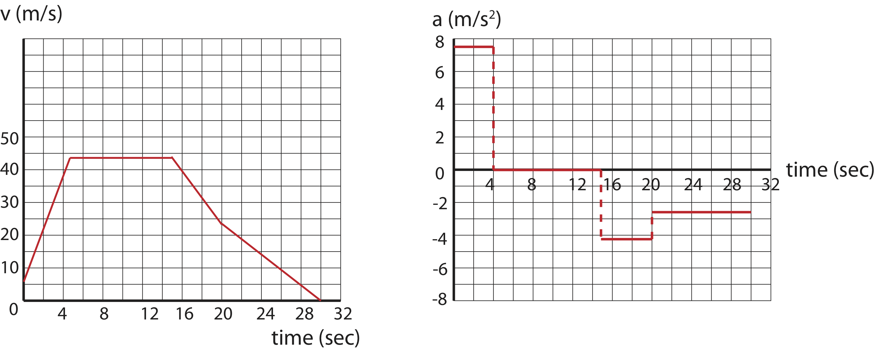
b) For the first 5 seconds, to find acceleration you need to calculate the x-component of gravity using the angle provided in the figure:
a=Fgxm=gsinθ=(9.8m/s2)(sin50∘)=7.51m/s2
The velocity is related to acceleration as:
a=ΔvΔt=vf−vitf−ti
The initial time is 0 seconds. Solving for vf at the bottom of the ramp, when tf=5sec:
vf=vi+atf=(6m/s)+(7.51m/s2)(5sec)=43.5m/s
Between 5 and 15 seconds acceleration is zero since there is no net force, so velocity remains constant at 43.5 m/s. Between 15 and 20 seconds the net forces points in the negative x-direction:
a=Fgxm=−gsinθ=−(9.8m/s2)(sin25∘)=−4.14m/s2
Solving for vf at 20 seconds at the top of the ramp:
vf=vi+a(tf−ti)=(43.5m/s)+(−4.14m/s2)(20sec−15sec)=22.8m/s
Between 20 and 30 seconds, we don't know the magnitude of the force, but we know that the train stops at 30 seconds:
a=vf−vitf−ti=0−22.8m/s30sec−20sec=−2.28m/s2
All of these calculations are summarized in the graphs below.
In this section we focused on depicting and interpreting motion graphically. In the next section, we will develop mathematical equations which will equivalently describe the motion and allow for more exact calculations of velocity and position at specific instances of time.
Contributors
Authors of Phys7B (UC Davis Physics Department)