8.2: Kinematics

Constant Acceleration

We have mostly focused so far on the source of acceleration, the forces, and what happens after the force acted on a system. Now we will look at the details of what happens to the motion of a system during the interaction, knows as kinematics. We will look at equations of motion for a specific case of constant acceleration. For example, an object in free fall near the surface of the Earth experiences constant acceleration due to gravity. Many other physical situations can be modeled by assuming the acceleration is constant. In this model, there are simple algebraic expressions relating the motion variables that make it convenient to get quantitative answers. Specifically, we are interested to get expression of velocity and position as a function of time. Even when acceleration is not constant over the entire range of motion, it is often possible to model the motion by considering acceleration to be constant over select intervals of time.

The algebraic equations for constant acceleration can be obtained by starting with the definition of acceleration:

\[a=\frac{dv}{dt}\]

To obtain the dependence of velocity on time, we need to change the above equation into integral form, and then set \(a\)= constant. You can check the results by differentiating the resulting expression. Integrating from some initial time, \(t_o\), to some later time, \(t\), to solve for change in velocity over time:

\[\Delta v=\int_{t_o}^{t} a dt\label{dv}\]

In general, when acceleration is not constant over time, the above integral can become complex. When acceleration is constant over time: 

\[a(t)=a\]

then it simply comes out of the integral in Equation \ref{dv}. Defining the change in velocity as, \(\Delta v=v_f-v_o\), where \(v_o\) is the velocity at some initial time \(t_o=0\), and \(v_f\) is velocity as time later time \(t\). Equation \ref{dv} becomes:

\[v_f=v_o+at\label{vt}\]

We can follow a similar procedure to determine how position varies with time for the case of constant acceleration. Starting with definition of velocity:

\[v=\frac{dx}{dt}\]

and integrating to solve for change in position over time:

\[\Delta x=x_f-x_o=\int_{0}^{t} v dt\label{dx}\]

Plugging in Equation \ref{vt} into the above equation we get:

\[x_f=x_o+\int_{0}^{t}(v_o+at) dt\]

Integrating we obtain the following expression for position as a function of time:

\[x_f=x_o+v_ot+\frac{1}{2}at^2\label{xt}\]

Equations \ref{vt} and \ref{xt} for velocity and position as a function of time can provide all the needed information about the motion of an object at constant acceleration. These equations of motion enable us to determine the position and velocity of an object at all times. 

When we derived the equations of motion, we assume that the motion is one-dimensional. At the end of this section, you will see how to us equations of motion when the motion is in two-dimensions. But even with one-dimensional motion velocity have a direction which means that the numerical value of \(v\) can be either positive or negative depending on the direction of motion. The position, \(x\), can also have an either positive or negative value, which will depend of the location of the object relative to the defined origin. Thus, it is important before starting to solve any kinematics problem to define the origin and assign a sign to each direction. By convention, typically to the right and upward from the origin is positive and to the left and downward from the origin is negative, but you might choose a different convention for convenience. There are many variables to keep track of, so let us categorize them. 

The following variables are constants:

• \(x_o\): the initial position of the system at \(t=0\) which is based on the choice of origin. Often, it is convenient to define the origin at the location of the object at \(t=0\), such that \(x_o=0\).
• \(v_o\): the initial velocity of the system at \(t=0\), which can be zero, positive, or negative. 
• \(a\): the acceleration which is a constant by definition, since these equations of motion are only valid when acceleration is constant. It can also be zero, positive, or negative. 

The following are independent variables:

• \(x_f\): the position of the system at some later time \(t\).
• \(v_f\): the velocity of the system at some later time \(t\).

The following is a dependent variable:

• \(t\): some later time, \(t>t_o\) during which one you aim to calculate \(x_f\) and \(v_f\).

Although Equations \ref{vt} and \ref{xt} are sufficient to provide all the information about the kinematics of an object as constant acceleration, another equation is often used for convenience, since it does not contain the time variable. This equation has the following form:

\[v_f^2-v_o^2=2a(x_f-x_o)\label{v-sq}\]

It it left up to you to show that the above equation comes from the two equations of motion in the following example.

Example \(\PageIndex{1}\)

Show that Equation \ref{v-sq} comes directly from Equations \ref{vt} and \ref{xt}.

Solution

In order to eliminate time from the combination of the two equations, let us solve for time using Equation \ref{vt} and plug the resulting for \(t\) into Equation \ref{xt}. We choose to do so in this order since Equation \ref{vt} depends only linearly on time. Solving to \(t\) using using Equation \ref{vt} we get:

\[t=\frac{v_f-v_o}{a}\nonumber\]

Plugging in the above result into Equation \ref{xt} we get:

\[x_f=x_o+v_o\Big(\frac{v_f-v_o}{a}\Big)+\frac{1}{2}a\Big(\frac{v_f-v_o}{a}\Big)^2\nonumber\]

Separating \(x\) and \(v\) on each side on the equation:

\[x_f-x_o=\frac{v_fv_o-v_o^2}{a}+\frac{1}{2a}(v_f^2-2v_fv_o+v_o^2)\nonumber\]

Simplifying we arrive at:

\[x_f-x_o=\frac{v_f^2-v_o^2}{2a}\nonumber\]

And finally rearranging the above equation to obtain the form of Equation \ref{v-sq} we arrive at:

\[v_f^2-v_o^2=2a(x_f-x_o)\nonumber\]

It is important to remember that these equations are valid when acceleration is constant which occurs when the net force is constant. A common example is free fall since the gravitational force on an object near the surface of the Earth is approximately constant. But even a freely falling object does not always experience constant acceleration when the effects of air friction become significant, such as a falling parachute. In that case, it is even possible to have zero acceleration, when air friction balances gravity, and the system reaches at terminal velocity.  However, there are many situations where acceleration is never constant. A mass hanging on a spring oscillating up and down represents a common situation where the acceleration is certainly not constant. The force changes as the mass oscillates, changing direction to pull the system toward equilibrium and increasing in magnitude as the mass goes further from equilibrium.

One-Dimensional Motion

We will now look at an example of an object falling near the surface of the Earth, in the case when the motion is in one-dimension, vertical motion only. If air friction on the object is sufficiently small compared to the pull of the Earth, we can model the situation as if only the force of gravity acts on the object. The object is said to be in free fall. For any object in free fall on the Earth, regardless its mass, its acceleration is equal to the gravitational constant: \(a=-g=-9.8 m/s^2\). The minus sign implies that acceleration is downward toward the center of the Earth, which by convention is a negative direction. In general, the object can have velocity of any direction, up, down, sideways, or something in between, but acceleration is always pointing down.

Figure 8.2.1 shows the free-body diagram for an object in free fall moving down. It also illustrates a diagram of position and velocity of the object at equal intervals of time.

Figure 8.2.1: An object in Free Fall

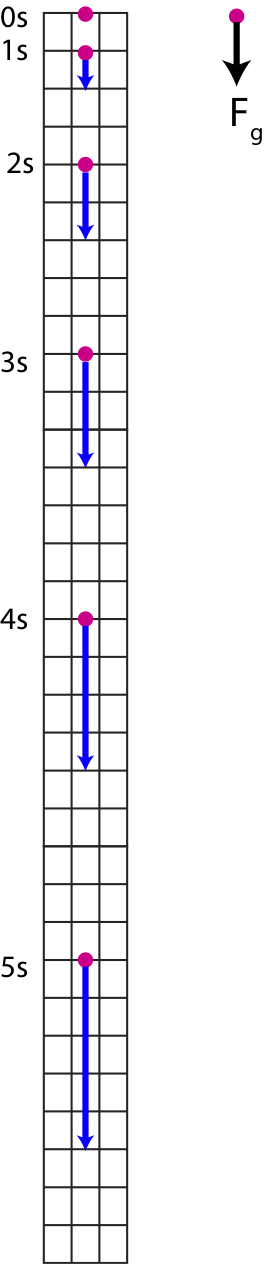
We assume that the object is stationary at \(t=0\), right before it is dropped. The blue arrows pointing down in the diagram specify the objects. Based on Equation \ref{vt} the velocity of an object in free fall changes according to:

\[v=-gt\]

where we set \(v_o=0\) for this example. Thus the velocity of the object increases linearly with time: 

\[\begin{array}{l} t=1 s:~~ v=-g \\ t=2 s:~~ v=-2g \\ t=3 s:~~ v=-3g\\ t=4 s:~~ v=-4g\\ t=5 s:~~ v=-5g\\~~~~~~~~~~~~\text{...}\end{array}\] 

The linear increase in velocity is indicated by the lengths of the blue arrows in Figure 8.2.1, the length of the first arrow is 1 unit, the second one is 2 units, the third is 3 units, and so on.

Based on Equation \ref{xt} position changes quadratically with time: 

\[x=-\frac{1}{2}gt^2\]

where we set \(x_o=0\) at the location of where the object is dropped, and \(v_o=0\) as before. The position of the object will be negative since it's moving down below the origin. Writing out the quadratic behavior for the first 5 seconds we get:

\[\begin{array}{l} t=1 s:~~ x=-\frac{1}{2}g \\ t=2 s:~~ x=-\frac{4}{2}g \\ t=3 s:~~ x=-\frac{9}{2}g\\ t=4 s:~~ x=-\frac{16}{2}g\\t=5 s:~~ x=-\frac{25}{2}g\\~~~~~~~~~~~~\text{...}\end{array}\] 

You can see this quadratic increase in position in Figure 8.2.1, since the dots representing the location of the object at equal intervals of time get further and further apart. 

Since position depends quadratically on time, the quadratic equation is often needed to solve for time. Rewriting Equation \ref{xt} in the form of a quadratic equation we get:

\[\frac{1}{2}gt^2+v_ot+(x_o-x_f)=0\]

Applying the quadratic equation to solve for time:

\[t=\frac{-v_o\pm\sqrt{v_o^2-2g(x_o-x_f)}}{g}\]

Although, the quadratic equation has two solutions, both of them are not always valid. If one of the solutions results in negative time, then that solution is not physical since time is always positive. However, sometimes two solutions are possible. Imagine you throw an object upward, and you want to know how long it takes it to get to a specific height, which is less than its maximum height. In this case there are two possible answers: the time it takes for the object to get to that height on the way up, and then the other solution is time it takes for the object to go all the way up and back down to that specific height.

Example \(\PageIndex{2}\)

The starting conditions of two cars at \(t=0\) are shown in the figure below. The green car, G, starts out 2 m ahead of the pink car, P. At \(t=0\) the pink car is moving to the right at 2 m/s, while the green car is moving to the right at 5 m/s. The pink car is accelerating to the right with magnitude of 6 m/s², while the green car is accelerating to the left with with magnitude of 4 m/s². Assume acceleration is constant for both cars. Define the origin at the location of the pink car at \(t=0\).

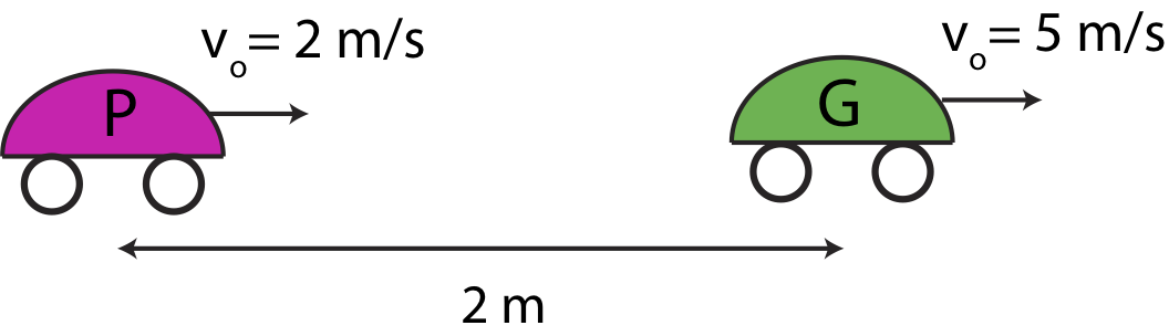
a) Calculate the time when the pink car catches up to the green one.

b) At which positions do the two cars meet?

Solution

a) We will use subscripts "P" and "G" to refer to the variables of the pink and green car, respectively. The pink car catches up to the green one when they are at the same location:

\[x_{f,P}=x_{f,G}\nonumber\]

Using Equation \ref{xt} for each car and setting them equal to each other we get:

\[x_{o,P}+v_{o,P}t+\frac{1}{2}a_Pt^2=x_{o,G}+v_{o,G}t+\frac{1}{2}a_Gt^2\nonumber\]

Moving all terms to the left-hand side of the equation and combining terms based on their dependence on \(t\) we get:

\[\frac{1}{2}(a_P-a_G)t^2+(v_{o,P}-v_{o,G})t+(x_{o,P}-x_{o,G})=0\nonumber\]

Let us now plug in all the constants for each car. By definition the pink car is at initially the origin,\(x_{o,P}=0\). If we define to the right as positive, then \(a_P=6~\textrm{m/s}^2\) and \(a_G=-4~\textrm{m/s}^2\). Substituting these values and the initial velocities given into the last equation we get:

\[\frac{1}{2}(-6-4)t^2+(2-5)t+(0-2)=0\nonumber\]

The above equation has the form of a quadratic equation:

\[0=5t^2-3t-2\nonumber\]

Solving the quadratic equation:

\[t=\frac{3\pm\sqrt{3^2-(4)(5)(-2)}}{(2)(5)}=\frac{3\pm 7}{10}=1, -\frac{2}{5}\nonumber\]

Since time cannot be negative, the two cars meet at \(t=1 s\).

b) Now we simply need to solve to the position of either car at \(t=1 s\). Solving for the pink car we get:

\[x_{f,P}=x_{o,P}+v_{o,P}t+\frac{1}{2}a_Pt^2=(2 m/s)(1 s)+\frac{1}{2}(6 m/s^2)(1^2s^2)=5 m\nonumber\]

To check that we get the same position for the green car at \(t=1 s\):

\[x_{f,G}=x_{o,G}+v_{o,G}t+\frac{1}{2}a_Gt^2=2m+(5 m/s)(1 s)+\frac{1}{2}(-4 m/s^2)(1^2s^2)=5 m\nonumber\]

Thus, the two cars meet 5 m to the right of the pink car's initial position.

Two-Dimensional Motion

When the object is moving in two-dimensions, we still use the same kinematics equations developed above, treating each direction independently. These kinematic equations for each spatial direction are summarized in the table below.

Table 8.1.1: Kinematics Equations in 2D

Description	Horizontal Direction, x	Vertical Direction, y
Constant Acceleration	\(a_x(t)=a_x\)	\(a_y(t)=a_y\)
Velocity as a function of time	\(v_{f,x}=v_{o,x}+a_xt\)	\(v_{f,y}=v_{o,y}+a_yt\)
Position as a function of time	\(x_f=x_o+v_{o,x}t+\frac{1}{2}a_xt^2\)	\(y_f=y_o+v_{o,y}t+\frac{1}{2}a_yt^2\)
Time independent equation	\(v_{f,x}^2-v_{o,x}^2=2a_x(x_f-x_o)\)	\(v_{f,y}^2-v_{o,y}^2=2a_y(y_f-y_o)\)

One common example of 2D motion is projectile motion, a object in free-fall whose initial velocity has a component in the horizontal direction. Since the object is in free-fall, it is still implies that the only force acting on it is the force of gravity pointing down. Thus, the equations in the table above can be simplified for projectile motion in the following way:

\[\begin{array}{l} a_x=0; && a_y=-g\\v_{f,x}=v_{o,x}; && v_{f,y}=v_{o,y}-gt \\ x_f=x_o+v_{o,x}t;&&y_f=y_o+v_{o,y}t-\frac{1}{2}gt^2\\v_{f,x}=v_{o,x};&&v_{f,y}^2=v_{o,y}^2-2g(y_f-y_o)\end{array}\label{pr}\]

The equations above state the motion in the x-direction remains constant since there is no net force in the x-direction: the x- component of velocity is constant and position in the x-direction changes linearly with time. In the y-direction the object follows the standard free-fall motion, as depicted in Figure 8.2.1. Projectile motion is illustrated in Figure 8.1.2 below, where initially the object has velocity pointing northeast, with some angle \(\theta\) above the positive x-axis.

Figure 8.1.2: Projectile Motion

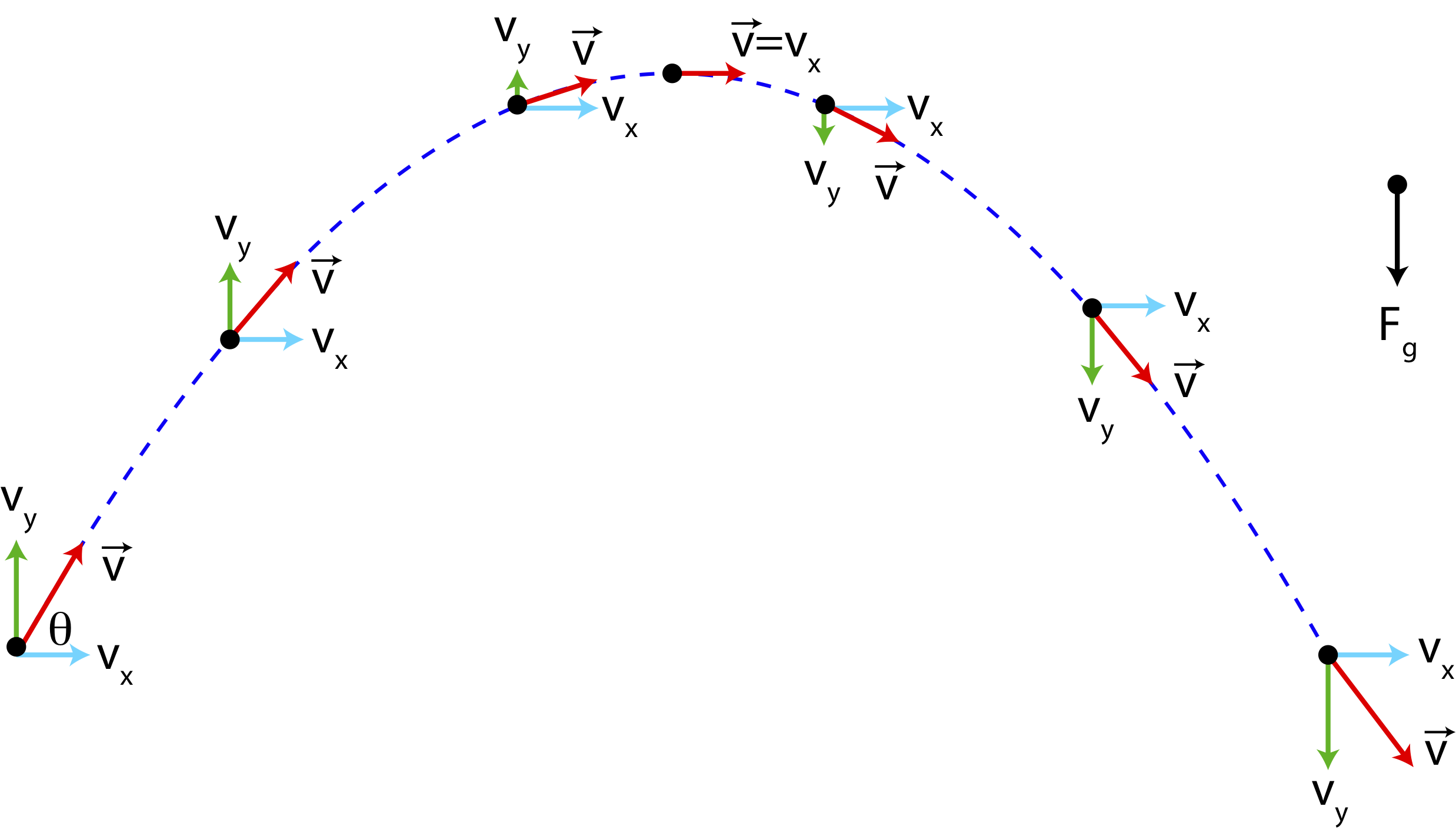
Since there is no force in the x-direction, which means that the component of velocity, \(v_x\), will be constant in this trajectory (light blue arrow marked \(v_x\) stays the same length throughout the motion). In the y-direction there is acceleration due to the force of gravity. Since the vertical component of initial velocity points up, the y-component of velocity will first decrease, then reach zero, and increase downward as the object starts moving down. Note, that this motion in the y-direction is identical to one-dimensional motion of an object being thrown directly upward. The fact that the object is also moving horizontally does not influence its vertical motion, since the two spatial direction are independent.

You can calculate the maximum height of the object in projectile motion using the last row in Equation \ref{pr}. At maximum height the speed in the vertical direction is zero, \(v_{f,y}=0\). Setting the initial height to zero, \(y_o=0\) and solving for the final height we get:

\[y_{max}=\frac{v_{o,y}^2}{2g}\label{ymax}\]

Recall from 7A, that this is the same result you would obtain from energy conservation:

\[\begin{array}{c}\Delta KE+\Delta PE = 0\\ \frac{1}{2}m(v_{max}^2-v_o^2)+mg(y_{max}-y_o) = 0\\-\frac{1}{2}v_o^2+gy_{max} = 0 \end{array}\]

The last line in the last equation is identical to the result in Equation \ref{ymax}. When it comes to calculating positions and speeds at different times, conservation of energy can give us the same results. However, conservation of energy model is limited since it cannot provide the details of the dynamics, such as the time it took for a certain motion or the direction of motion. Thus, we need to turn to Newton's Laws and kinematics to answer those questions.

For example in order to calculate the amount of time it takes for the object to return to its initial height, \(y_f=y_o\), you need to use kinematics:

\[0=v_{o,y}t-\frac{1}{2}gt^2\]

This equation have two solutions:

\[t=0,t=\frac{2v_{o,y}}{g}=\frac{2v_o\sin\theta}{g}\label{time-tot}\]

Of course, the \(t=0\) solution just specifies the initial time, so the second solution tells us how long it would take to return to the same height. To obtain this time, we did not use any information about the motion in the x-direction. So if you throw an object straight up and another object at an angle with the same initial vertical speed, the two objects would land back on the ground at the same time even though one of the objects traveling in the horizontal direction as well. To calculate how far it would land from its initial position we can use the expression for position in Equation \ref{pr} in the x-direction and the time obtained in Equation \ref{time-tot}:

\[x_f=x_o+v_{o,x}t=(v_o\cos\theta)\Big(\frac{2v_o\sin\theta}{g}\Big)=\frac{2v_o^2\cos\theta\sin\theta}{g}=\frac{v_o^2\sin(2\theta)}{g}\]

where in the last step we used a trigonometric identity. The equation above tells that that the faster the object is moving the further it will travel horizontally. If the angle is \(90^{\circ}\), the motion is purely vertical, so the horizontal displacement will be zero. When the angle is \(0^{\circ}\), again we get a displacement of zero since we are looking for "an arc" when we calculated the time for the object to come back to the same height. Of course, you can throw an object purely horizontally from above the ground, and it would land some distance away. But it would never be at the same height again, since that's equivalent to an object being dropped down.

Example \(\PageIndex{3}\)

Below is a diagram ball 1 being thrown at an angle \(\theta=40^{\circ}\) above the horizontal at a height of \(h=1.5 m\) above the ground. The initial speed of ball 1 is 10 m/s. Ball 2 is thrown from the ground directly upward, a distance \(d=2 m\) to the right of ball 1.

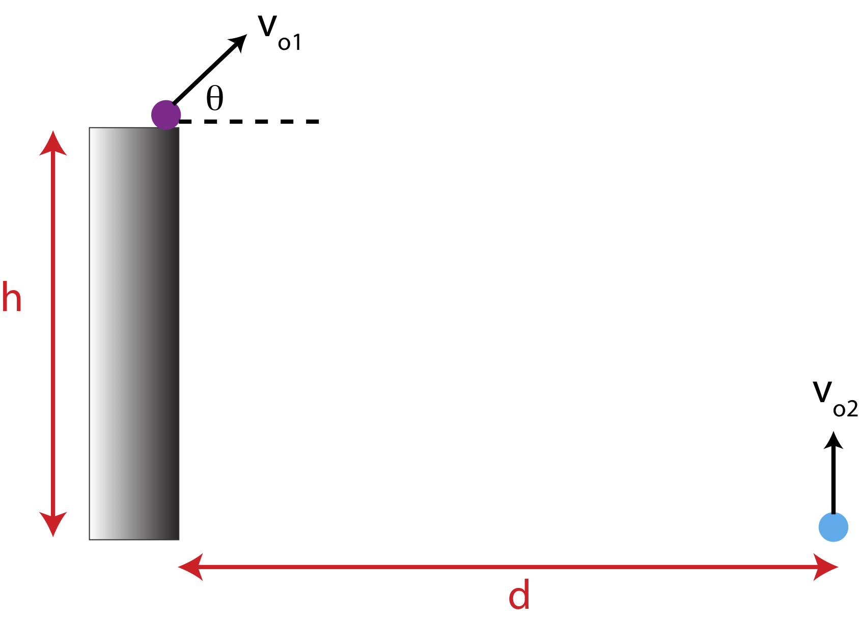
a) The two balls collide as ball 2 travels up. Find the time when the two balls collide, and the speed at which ball 2 is thrown upward.

b) If the two balls did not collide and ball 1 continued on its trajectory, calculate the velocity of ball 1 right before it reaches the ground.

Solution

The time at which the balls collide is the time that it takes the first ball to move by distance d horizontally. Setting \(x=0\) at the initial location of ball 1 we get:

\[d=v_{o1,x}t=(v_{o1}\cos\theta)(t)\nonumber\]

Solving for time:

\[t=\frac{d}{v_{o1}\cos\theta}=\frac{2m}{(10 m/s)(\cos 40^{\circ})}=0.261 s\nonumber\]

The height of both balls at this time is:

\[\textrm{ball 1}:~~y_1=h+v_{o1}\sin\theta t-\frac{1}{2}gt^2\nonumber\]

\[\textrm{ball 2}:~~y_2=v_{o2}t-\frac{1}{2}gt^2\nonumber\]

Setting them equal to each other:

\[h+v_{o1}\sin\theta t-\frac{1}{2}gt^2=v_{o2}t-\frac{1}{2}gt^2\nonumber\]

\[v_{o2}=\frac{h}{t}+v_{o1}\sin\theta=\frac{1.5 m}{0.261 s}+(10 m/s)(\sin 40^{\circ})=12.2 m/s\nonumber\]

b) Since there is no force in the x-direction, the component of velocity in the x-direction will remain the same:

\[v_{fx}=v_{ox}=v_{o1}\cos\theta=(10 m/s)(\cos 40^{\circ})=7.66 m/s\nonumber\]

We don't need to solve for time directly, thus, it is convenient to use the kinematics equation which does not depend on time to directly calculate the y-component of velocity when the ball reaches the ground, \(y_f=0\):

\[v_{f,y}^2=v_{o,y}^2+2a_y(y_f-y_o)\nonumber\]

Solving for \(v_{f,y}\):

\[|v_{f,y}|=\sqrt{[(10 m/s)(\sin40^{\circ})]^2+2(-9.8 m/s^2)(0-1.5m)}=8.41 m/s\nonumber\]

This is the absolute value of the velocity, but the componet is negative since the ball is moving downward before it hits the ground:

\[\vec v_f=(7.66,-8.41) m/s\nonumber\]

Solving for magnitude:

\[|\vec v_f|=\sqrt{7.66^2+8.41^2}=11.4 m/s\nonumber\]

And angle:

\[\theta_f=\arctan\Big(\frac{8.41}{7.66}\Big)=47.7^{\circ}\nonumber\]

moving down in the southeast direction.

Contributors

• Authors of Phys7B (UC Davis Physics Department)