2.6: Static Networks

Symbolic Diagrams

We have discussed capacitors as theoretical constructs, but in fact they are common electrical components, used in many devices. One typical use is as a source of a “burst” of electrical energy that is stored when a voltage source charges it at its leisure, but then is unleashed more quickly to do some job that the original voltage source cannot supply so fast. We will see more uses as well, in a later chapter. To discuss capacitors in this practical context, it becomes helpful to introduce some symbolic notation. We start with four symbols:

equipotential: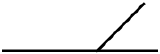

Solid, unbroken lines that connect components represent equipotentials. These can consist of single lines, or lines that branch-off from each other. While it is usually harmless to do so, thinking of these lines as conducting wires in the physical world can sometimes be dangerous when they are first encountered, as we will use this same set of symbols later when we discuss electric current, where wires are not equipotentials. Also, problems are easier to solve if you keep in mind that everything connected by straight lines are at the same potential, rather than just a conduit of charge flow.

switch: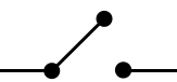

This is a component that facilitates talking about processes that involve connecting and disconnecting other components. When the switch is closed, it simply becomes an equipotential.

capacitor: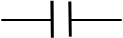

The symbol looks like the side view of a parallel-plate capacitor, but it can represent any geometry of capacitor, with or without a dielectric within it. Note that the connection of a "plate" with a straight line suggests that they are at the same potential (and they are), but because there is a gap between the two plates, they are of course not at the same potential. This is the first of many components we will encounter that generally involve a potential difference from one side to the other.

battery:

Up to now, we have talked about "holding a capacitor at a constant potential difference," while we do such things as pull the plates apart or insert a dielectric. We will no longer require this cumbersome language, as this is precisely the function of a battery. When charges move into or out of a capacitor, the potential difference (or voltage) across the plates changes, but the two "plates" of the battery shown in the symbol remain at the same potential difference at all times. If one side of the battery is connected by an equipotential to one side of a component, then that side of the component remains at the potential provided by the battery. If maintaining this potential requires charge movement, the battery supplies or accepts the charge as needed. [It should be noted that there are several symbols one may encounter for batteries. The '–" and '+' in the symbol shown are actually superfluous and don't always appear – the larger "plate" is always the one at higher potential. Also, a symbol with more than just two "plates" (alternating in size) is often used for a battery.]

Equivalent Capacitance

Next we will combine multiple components together, connected by equipotentials. A circuit is a closed-loop of components and equipotentials. Often these systems of components involve branching equipotentials, which results in many closed loops. Such a system is a combination of many circuits, and often the entire system referred to collectively as a circuit as well, but a more precise term for such a system is network. The reader is likely to encounter both terms to describe such systems in this work.

In order to analyze these systems, it is useful to develop some tools for examining circuit fragments of multiple capacitors (each of which can have a different capacitance). The simplest such fragment is one in which they are connected "consecutively," as shown in the figure below.

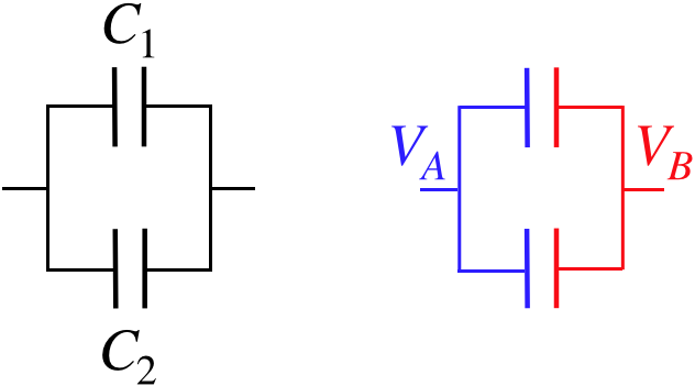
Figure 2.6.1 – Capacitors in Series

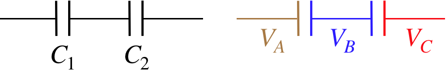
The color-coded diagram on the left emphasizes the equipotentials and plates that are all at the same potential – the left plate of capacitor #1 is at potential \(V_A\), the right plate of capacitor #1 and the left plate of capacitor #2 are at potential \(V_B\) and the right plate of capacitor #2 is at potential \(V_C\). The voltage across the capacitors are therefore:

\[V_1 = V_A-V_B\;,\;\;\;\;\;V_2=V_B-V_C \]

This means that the voltage difference between the equipotentials on the two ends of the combination of capacitors is simply the sum of the voltages across the capacitors:

\[V_{tot} = V_A-V_C = \left(V_A-V_B\right) + \left(V_B-V_C\right) = V_1+V_2\]

What about the charge on each capacitor? Well, we know that the plates on a single capacitor have equal charge with opposite signs. The blue segment is isolated, so cannot receive any outside charge, which means that whatever charge is on the right plate of capacitor #1, the same amount of charge with the opposite sign is on the left plate of capacitor #2. Therefore the charge on each capacitor in this configuration is the same.

Whenever two or more capacitors are arranged in this way, such that they satisfy the above properties (the voltage across the combination is the sum of the voltages of each one, and the charges are the same on all of them), we say that these capacitors are in series. We have a total voltage difference for the combination, and a single amount of charge on a plate, so we can define an equivalent capacitance for the arrangement. Specifically:

\[\left. \begin{array}{l} Q=C_{eq}V_{tot} \\ Q=C_1V_1 \\ Q=C_2V_2 \\ V_{tot}=V_1+V_2 \end{array} \right\}\;\;\; \dfrac{1}{C_{eq}} = \dfrac{1}{C_1} + \dfrac{1}{C_2} \;\;\;\text{(series)}\]

Note that if there are more than two capacitors in series, we only need to add additional inverse terms.

Alert

It is not uncommon to mistakenly declare capacitors to be in series, simply because they "look consecutive," when in fact they are not in series. It is important to make sure that the criteria involving voltage and charge are in effect before computing an equivalent series capacitance.

Another basic arrangement of capacitors reverses the roles of charge and voltage, and is shown in the figure below.

Figure 2.6.1 – Capacitors in Parallel

Once again the right diagram color-codes the equipotentials, and this time we can see that the two capacitors have the same potential difference across them:

\[V_1 = V_A-V_B = V_2\]

As for the charge, each plate must get charge from outside (through the equipotentials), and different amounts of charge will go to the capacitors, and the total charge supplied to this system will equal the sum of the charges supplied to each individual capacitor. When these two criteria hold, we say that the capacitors are in parallel.

Alert

This is another warning about declaring two capacitors to be in parallel, simply because they look like it. The simplest test for parallel capacitors is to check to see if an equipotential directly connects both plates of one capacitor to the corresponding plates of the other capacitor.

For an equivalent capacitance, we put together the two new criteria, and get a new relation:

\[\left. \begin{array}{l} Q_{tot}=C_{eq}V \\ Q_1=C_1V \\ Q_2=C_2V \\ Q_{tot}=Q_1+Q_2 \end{array} \right\}\;\;\; C_{eq} = C_1 + C_2\;\;\;\text{(parallel)}\]

If there are more than two capacitors in parallel, then of course the equivalent capacitance is the sum of all the individual capacitances.

Example \(\PageIndex{1}\)

Show that for both the series and parallel cases, the energy stored in the equivalent capacitor equals the sum of the energies in the individual capacitors.

Solution

For the series case, the charge is the same on both capacitors, so the total stored energy is:

\[U = U_1 + U_2 = \dfrac{Q^2}{2C_1} + \dfrac{Q^2}{2C_2} = \dfrac{Q^2}{2}\left(\dfrac{1}{C_1}+\dfrac{1}{C_2}\right)=\dfrac{Q^2}{2C_{eq}} \nonumber\]

For the parallel case, the voltage is the same across both capacitors:

\[U = U_1 + U_2 = \frac{1}{2}C_1V^2 + \frac{1}{2}C_2V^2 = \frac{1}{2}\left(C_1+C_2\right)V^2=\frac{1}{2}C_{eq}V^2 \nonumber\]

Networks of Capacitors

Now just because we only have an equation for a pair of capacitors, it doesn’t mean that we can only solve problems with two capacitors. We can solve much bigger networks, in a bootstrap manner by combining pairs of capacitors to form equivalent capacitors, then treating equivalent capacitors as if they are "real" capacitors, and combining them into new equivalent capacitors. Once enough reductions have occurred, one can conclude how much charge comes off the battery, and then "work backwards," keeping in mind that the amount of charge on an equivalent capacitor is the same as the charge on its constituent capacitors if they are in series, and the voltage difference across the equivalent capacitor is the same as across its constituent capacitors if they are in parallel. Once all the equivalent capacitors have been unwound, the charges and voltages (and therefore the energies as well) are known for every capacitor in the network. Mastering this process is only a matter of practice, so here's an example...

Example \(\PageIndex{2}\)

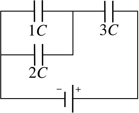
For the network in the figure, compute the fraction of the total energy supplied by the battery that goes to each of the individual capacitors.

Solution

We will begin by calling the voltage across the battery '\(V\)'. It will divide out of the final answer, but we need something to put into the algebra. Now we begin the process of combining the capacitors to create a single equivalent capacitance for the network.

It might seem like \(1C\) and \(3C\) are in series, but they are not! The equipotential that connects to the left plate of \(3C\) splits and connects to the right plates of two capacitors. This means that the sum of the charges on the right plates of \(1C\) and \(2C\) is the negative of the charge on the left plate of \(3C\). With the charges not equal for \(1C\) and \(3C\), they cannot be in series. On the other hand, tracing the equipotential attached to the left plate of \(1C\) goes to the left plate of \(2C\), while tracing the equipotential attached to the right plate of \(1C\) goes to the right plate of \(2C\), so they have equal voltage drops and are in parallel. We replace them with an equivalent capacitance (which is just the sum of their capacitances), and redraw the diagram:

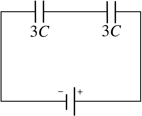
These capacitors are clearly now in series, so we combine them to make a single equivalent capacitor:

\[\dfrac{1}{C_{eq}} = \dfrac{1}{C_1} + \dfrac{1}{C_2} = \dfrac{2}{3C}\;\;\;\Rightarrow\;\;\; C_{eq} = \frac{3}{2}C\nonumber\]

With a single equivalent capacitor attached to the battery, we can compute how much charge leaves the battery, and the amount of energy supplied by the battery:

\[\begin{array}{l} Q_{tot} = C_{eq}V = \frac{3}{2}CV \\ U_{tot} = \frac{1}{2}C_{eq}V^2 = \frac{3}{4}CV^2 \end{array} \nonumber\]

Now comes the tricky part – the "unwinding." We start with the charge supplied by the battery. Whatever positive charge leaves the battery collects on the right plate of \(3C\) - it can't go anywhere else. This tells us immediately the voltage across \(3C\), and from that, the energy stored on it.

\[\begin{array}{l} Q_3 = Q_{tot} = \frac{3}{2}CV && \Rightarrow && V_3 = \dfrac{Q_3}{3C} = \frac{1}{2}V \\ U_3 = \frac{1}{2}\left(3C\right)V_3^2 && \Rightarrow && U_3 = \frac{3}{8}CV^2 \end{array} \nonumber\]

The equivalent capacitor for \(1C\) and \(2C\) is in series with \(3C\), so the sum of their voltages must equal the total voltage across the combination, which is just the voltage of the battery. Therefore, unsurprisingly, the voltage across equivalent capacitor for \(1C\) and \(2C\) is also \(\frac{1}{2}V\). The two individual capacitors in this parallel combination have the same voltage differences as the voltage difference of their combination, so we can compute the energy stored in each of these (we don't need to compute the charge on each capacitor, but we could easily do so, if we wanted)

\[\begin{array}{l} U_1 = \frac{1}{2}\left(1C\right)CV_1^2 = \frac{1}{2}\left(1C\right)C\left(\frac{1}{2}V\right)^2 = \frac{1}{8}CV^2 \\ U_2 = \frac{1}{2}\left(2C\right)CV_2^2 = \frac{1}{2}\left(2C\right)C\left(\frac{1}{2}V\right)^2 = \frac{1}{4}CV^2 \end{array}\nonumber\]

The fractions of energy stored in each capacitor are therefore:

\[\begin{array}{l} \dfrac{U_1}{U_{tot}} = \dfrac{\frac{1}{8}CV^2}{\frac{3}{4}CV^2} = \dfrac{1}{6} \\ \dfrac{U_2}{U_{tot}} = \dfrac{\frac{1}{4}CV^2}{\frac{3}{4}CV^2}= \dfrac{1}{3} \\ \dfrac{U_3}{U_{tot}} = \dfrac{\frac{3}{8}CV^2}{\frac{3}{4}CV^2} = \dfrac{1}{2}\end{array}\nonumber\]

Note that these fractions add to 1, which confirms that the total energy that leaves the battery equals the sum of the energies in the three capacitors.

There are other applications of these tools that don't neatly fall into this template. These sorts of examples require some thought as to whether series or parallel applies. Here are a couple of the slightly-more-offbeat examples...

Example \(\PageIndex{3}\)

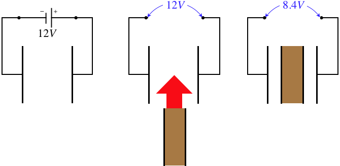
A parallel-plate capacitor with a vacuum between its plates is charged by connecting it to a 12V battery, and after it is fully charged, the battery is disconnected. Next an insulator with a thickness equal to half the width of the gap in the original capacitor is sandwiched between two thin conducting plates and is inserted between the plates of the original capacitor. After this is done, the voltage across the full system is measured to be 8.4V. Find the dielectric constant of the insulator.

Solution

Placing the dielectric between the plates creates three separate regions within the capacitor. Thanks to the electric field being perpendicular to the plates, each end of the dielectric is an equipotential, which means that we can treat the three regions as though they are separate parallel-plate capacitors which are in series. The center capacitor has a dielectric while the outer capacitors have vacuum gaps. For the sake of doing the math, we’ll call the gap size of the original capacitor \(2d\) (making the thickness of the dielectric \(d\) and the thicknesses of the outer two capacitors \(\frac{1}{2}d\). We'll call the area of the plates \(A\), and the dielectric constant (which we seek) \(\kappa\).

a. The capacitance of the original capacitor is:

\[C_{before} = \dfrac{\epsilon_oA}{2d}\nonumber\]

Treating the new configuration as three capacitors in series and computing the equivalent capacitance gives:

\[\dfrac{1}{C_{after}} = \dfrac{1}{C_1}+\dfrac{1}{C_2}+\dfrac{1}{C_3} = \dfrac{\frac{1}{2}d}{\epsilon_oA}+\dfrac{d}{\kappa\epsilon_oA} + \dfrac{\frac{1}{2}d}{\epsilon_oA} \;\;\;\Rightarrow\;\;\; C_{after} = \dfrac{\epsilon_oA}{d}\left[\dfrac{\kappa}{\kappa + 1}\right]\nonumber\]

With the plates disconnected from the battery, the charge on the capacitor plates remains constant through this process (it has nowhere to go!). Setting the charges equal gives us a ratio of the before and after capacitances in terms of the ratio of the given voltages:

\[Q=C_{before}V_{before}=C_{before}V_{before}\;\;\;\Rightarrow\;\;\; \dfrac{C_1}{C_2} = \dfrac{V_2}{V_1} \;\;\;\Rightarrow\;\;\; \dfrac{\dfrac{\epsilon_oA}{2d}}{\dfrac{\epsilon_oA}{d}\left[\dfrac{\kappa}{\kappa + 1}\right]} = \dfrac{\kappa+1}{2\kappa} = \dfrac{8.4V}{12V} \;\;\;\Rightarrow\;\;\; \kappa = 2.5\nonumber\]

Example \(\PageIndex{4}\)

Two capacitors are separately connected to batteries until they are fully charged, and then are disconnected. At this point the capacitors hold equal charge, but capacitor #1 stores three times as much energy as capacitor #2. The two capacitors are then connected to each other such that the positive lead of one capacitor is connected to the positive lead of the other, and likewise with the negative leads.

1. In which direction does charge flow when this connection is made, and what fraction of the charge flows out of the capacitor that loses charge?
2. If the voltage difference between the positive plates and negative plates after the capacitors are connected is \(V\), find the voltage across each capacitor before they were connected in terms of \(V\).
3. Find the fraction of energy change in the system when the charges rearrange themselves after the capacitors are connected. Is it a gain or a loss?

Solution

a. Start with the fact that both capacitors had equal charge, that we will call \(Q\). Then apply the fact that capacitor #1 stored three times as much energy:

\[U_1 = 3U_2 \;\;\;\Rightarrow\;\;\; \dfrac{Q^2}{2C_1}=3\dfrac{Q^2}{2C_2}\;\;\;\Rightarrow\;\;\;C_2 = 3C_1\nonumber\]

When they are connected together, it is in parallel, because the plates of one capacitor are connected to their counterparts on the other capacitor with equipotentials. This means their plates are now forced to be at the same potential difference. Two capacitors with equal voltage differences will hold charges proportional to their capacitances:

\[\left.\begin{array}{l} Q_1=C_1V \\ Q_2=C_2V \end{array} \right\}\;\;\; \dfrac{Q_1}{Q_2} = \dfrac{C_1}{C_2} \nonumber\]

So capacitor #2 will have 3 times as much charge on its plates as capacitor #1 when the charge stops rearranging itself. They started with equal charge, so for capacitor #2 to have 3 times as much charge as #1, #1 must have lost half its starting charge. In terms of our defined value \(Q\), capacitor #1 ends up with \(\frac{1}{2}Q\), while capacitor #2 ends up with \(\frac{3}{2}Q\).

b. We have the before and after conditions, and comparing them gives our answers:

\[\left.\begin{array}{l} before: && Q=C_1V_1 \\ after: && \frac{1}{2}Q = C_1V \end{array} \right\}\;\;V_1 = 2V\nonumber\]

\[\left.\begin{array}{l} before: && Q=C_2V_2 \\ after: && \frac{3}{2}Q = C_2V \end{array} \right\}\;\;V_2 = \frac{2}{3}V\nonumber\]

c. Writing the total energies before and after in terms of \(Q\) and \(V\) gives:

\[\begin{array}{l} before: && U=\frac{1}{2}QV_1 + \frac{1}{2}QV_2 = \frac{1}{2}Q\left(2V\right) + \frac{1}{2}Q\left(\frac{2}{3}V\right) = \frac{4}{3}QV \\ after: && U=\frac{1}{2}Q_1V + \frac{1}{2}Q_2V = \frac{1}{2}\left(\frac{1}{2}Q\right)V + \frac{1}{2}\left(\frac{3}{2}Q\right)V = QV \end{array}\nonumber\]

The system drops to three quarters of its original energy, so it loses one-fourth of what it started with.

Where does the energy go? Just for the sake of argument, let's suppose the capacitors are of the parallel-plate variety, and that capacitor #2 has three times the capacitance of capacitor #1 because its plates have three-times the area. With equal charges on each capacitor, this means that the charge density on capacitor #1 is three times greater than on capacitor #2. The fact that the charges are squeezed together more tightly on capacitor #1 is the reason that more potential energy is stored there. Allowing the charges to redistribute uniformly by connecting the capacitors results in the system evolving to a lower potential energy state. In terms of forces, the repulsion of charges on capacitor #1 exceeds the repulsion of those charges from capacitor #2, so net work is done by the electrical force in reaching the new state (reducing the potential energy), and since we assume that the kinetic energy given to the charges is ultimately dissipated away, the energy in the system at the end is lower than at the start.