4.5: Ampère's Law

A Magnetic Analog to Gauss's Law for Electricity

We have already stated that Gauss's law for magnetic field is trivial, as there are no magnetic monopoles, but it turns out that there is a separate mathematical law that works for magnetic sources in the same way that Gauss's law works for electric sources. It incorporates "enclosed" sources, and allows us to use symmetrical situations to solve for fields using methods simpler than integrating Biot-Savart's law.

This magnetic version of the electrical Gauss's law is called Ampère's law, and since it can't involve enclosed point sources, it instead deals with lines of current, which either circle back on themselves to form a closed circuit, or are infinitely-long (and circle-back on themselves at infinity). But how do we "enclose" a line of current? In the case of charge, it was enclosed if there was no way to remove the charge from the Gaussian surface without breaking through the surface (i.e. the surface has no holes in it). In the case of Ampere's law, we consider a current to be enclosed by an imaginary closed path – called an Ampèrian circuit – rather than a surface. Such a current is enclosed when there is no way to move the line of current out without it breaking through the Ampèrian circuit.

Figure 4.5.1 – Defining an Enclosed Current

There are two ways that a current won't be enclosed: If there is a break in the path around the wire, so that the wire can slide through it, or is the segment of wire is finite in length and does not form a closed loop. If the loop of wire is closed, then the Ampèrian circuit is "linked" with it, and the current is enclosed. If the wire is infinitely long, the wire similarly cannot escape the Ampèrian circuit without breaking through it, so its current is also enclosed. [Mathematically, we generally define a current to be "enclosed" by a closed path if it pierces every possible surface that is bounded by the closed path. Clearly there are stretched surfaces we can construct with the closed path as it border that do not allow a finite-length segment to pierce it.]

With this definition of enclosed current in place, we have Ampère's law:

\[\oint \limits_{\rm {path}}\overrightarrow B \cdot \overrightarrow {dl} = \mu_oI_{enclosed}\]

The integral is performed along any Ampèrian circuit that goes completely around the enclosed current, in the same way that the integral for Gauss's law works for any closed surface that encloses the charge. All of the properties of Gauss's law have analogous properties for Ampère's law:

• Enclosed is defined in terms of ability to remove charge/current from surface/closed path without breaking through the enclosure.
• The sign of the charge inside a Gaussian surface is related to the positive direction of the area vector. If the total flux is in the negative direction (opposite to the area orientation), then the enclosed charge is negative. Similarly, we define a positive direction of circulation for an Ampèrian circuit, and if the direction of the magnetic field of the current has the same circulation orientation as that of the Ampèrian circuit, then that current is "positive," otherwise it is "negative."
• There can be both positive and negative charges/currents enclosed in a surface/closed path, and these are combined to give a net charge/current.
• We can use symmetry to solve for a field. This usually means that the field is either parallel or perpendicular to the surface/closed path, and that it has a constant magnitude on that surface/closed path.
• The shape of the surface/closed path is not relevant, as long as it is closed.

Figure 4.5.2 – Comparing Gauss's Law to Ampère's Law

Applications of Ampère's Law

The applications of Ampère's law are much like those of Gauss's law – symmetry is used to compute fields. Before we do any of these, let's confirm a result we already have – the field on the axis of a circular loop of radius \(r\) (Equation 4.4.10). We need to choose a useful circuit – it needs to enclose the current, and it needs to have a direction that matches well with the direction of the magnetic field that we know from symmetry. To this end, we will choose an Ampèrian circuit that follows the \(z\)-axis from \(-\infty\) to \(+\infty\), and from there circulates back around on itself at infinity. The integral of this infinitely-distant segment of the closed path will vanish, because the field weakens to zero this far away, so all that is left is the integral along the \(z\)-axis.

Figure 4.5.3 – Ampèrian Circuit for Loop

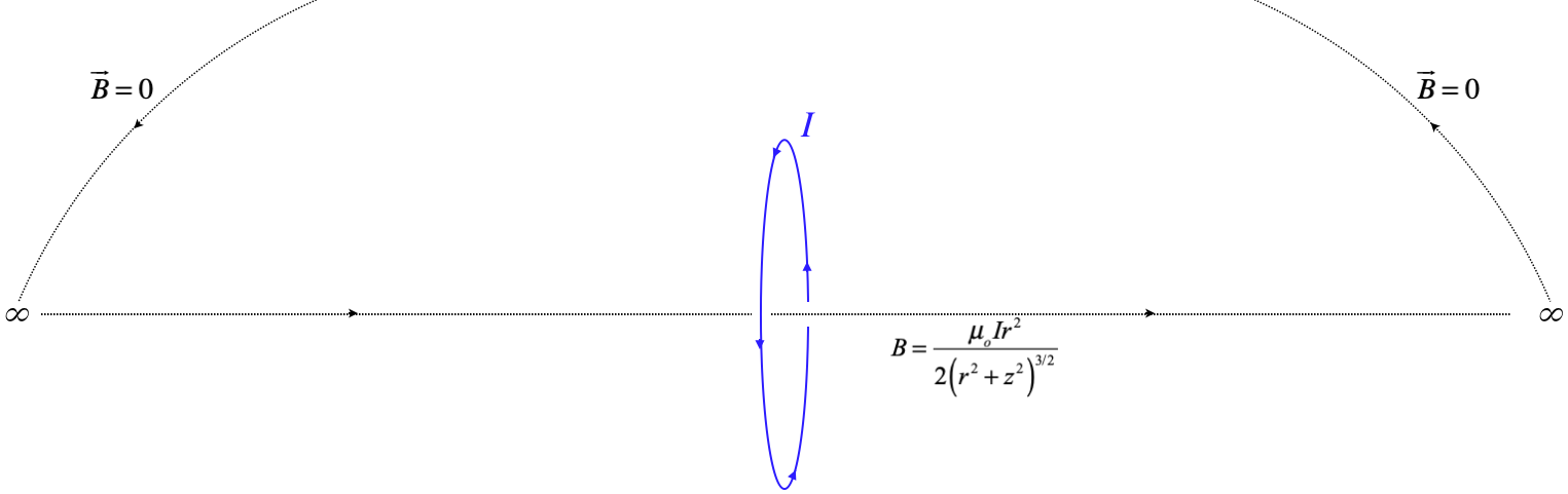
The magnetic field on the axis is in the same direction as the circuit along the \(z\) axis, and while we don't know the angle between the field and the direction of the path elsewhere, it doesn't matter, because the field vanishes. So the closed-path line integral gives:

\[\oint \overrightarrow B \cdot \overrightarrow {dl} = \int\limits_{z-axis} Bdz + \int\limits_{R=\infty}\overrightarrow B \cdot \overrightarrow {dl} = \dfrac{\mu_oIr^2}{2}\int\limits_{-\infty}^{+\infty} \dfrac{dz}{\left(r^2+z^2\right)^{\frac{3}{2}}} + 0 = \dfrac{\mu_oIr^2}{2}\left[\dfrac{z}{r^2\sqrt{r^2+z^2}}\right]_{-\infty}^{+\infty} = \mu_oI\]

Since the enclosed current within this Ampèrian circuit is in fact the current in the circular loop, and since this current has a positive orientation for this closed path (it is coming out of the page and the path is counterclockwise, satisfying the right-hand-rule), Ampère's law is confirmed for this case.

Next let's use Ampère's law in a more traditional fashion – to compute the magnetic field in a symmetric physical situation. We'll look at the field of a solenoid. The solenoid has a high degree of symmetry, mainly thanks to our assumption that it is essentially infinite in length. Consider the direction of the field inside the solenoid. There is no reason to expect that it would diverge from being parallel with the axis anywhere, because then what would make the point where this divergence occurs so special? It looks like every other point in the infinite solenoid, so the field direction should be the same as every other point in the solenoid. Furthermore, it should not get any stronger along the axis – why would the field be a greater magnitude at one point along the axis than any other?

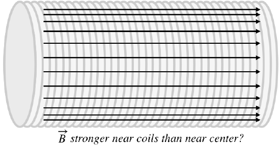
Of course, knowing that the field inside the solenoid is parallel to the axis everywhere and equal strength as a function of its position along the axis inside the solenoid doesn't tell us that the field strength is also uniform as a function of distance from the axis – perhaps it gets stronger as the position gets closer to the wire coils? For example, the field may look like this:

Figure 4.5.4 – Speculation About the Magnetic Field Inside a Solenoid

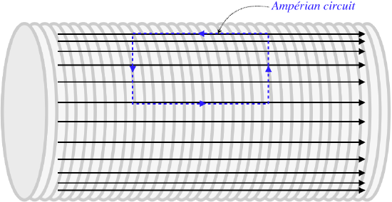
We can check this speculation using Ampère's law. We do this by constructing a rectangular Ampèrian circuit inside the solenoid that has two sides parallel to the field, and two sides perpendicular to the field.

Figure 4.5.5 – An Ampèrian Circuit for the Interior of the Solenoid

Now we apply Ampère's law. First of all, there is no electric current flowing through this closed path, so the integral around the path will be zero:

\[\oint \overrightarrow B \cdot \overrightarrow {dl} = \mu_oI_{enclosed} = 0\]

Second, the magnetic field is perpendicular to two of the sides of the rectangle, so the dot product of the field with the displacements during that portion of the circuit is zero, giving zero integral along the vertical segments. And the field strength doesn't change along the direction of the axis, while the field is parallel to these parts of the path, so the dot products and integrals are easy to perform:

\[\begin{array}{l} \int\limits_{vertical} \overrightarrow B \cdot \overrightarrow {dl} && = && 0 \\ \int\limits_{top} \overrightarrow B_{top} \cdot \overrightarrow {dl} && = && \int \left(-B_{top}\;dl\right) && = && -B_{top}L \\ \int\limits_{bottom} \overrightarrow B_{bottom} \cdot \overrightarrow {dl} && = && \int \left(+B_{bottom}\;dl\right) && = && +B_{bottom}L \end{array}\]

Adding all four contributions to the integral and setting it equal to zero (no enclosed current) gives us the result that \(B_{top} = B_{bottom}\), which means that the field strength at different distances from the axis inside the solenoid is actually the same. The magnetic field in the interior of a solenoid is completely uniform.

Notice that a rectangular Ampèrian circuit parallel to the axis drawn outside the solenoid must give us the same result: The magnetic field must be uniform out there as well. But that means that the field is the same strength infinitely-far from the solenoid as it is just outside of it. Naturally the field is zero infinitely-far away, which means that we can conclude that the magnetic field is zero everywhere outside the solenoid.

Finally, we can also use Ampère's law to determine the strength of the uniform magnetic field inside the solenoid, without going through the integration of an infinite number of loops, as we did in the previous section. We accomplish this by constructing a rectangular Ampèrian circuit parallel to the axis with one side inside the solenoid, and one outside of it.

Figure 4.5.6 – An Ampèrian Circuit to Compute Field Inside a Solenoid

As before, we see that the contributions to the integral by the vertical sides of the rectangular path are zero, because inside the solenoid the field is perpendicular to the path (and outside the solenoid the field is zero). This time, however, the contribution by one of the horizontal sides (the one outside the solenoid) is also zero, since there is no field. The side of the rectangle inside the solenoid is easy to integrate, so putting them all together into Ampère's law gives:

\[\mu_oI_{enclosed}=\oint \overrightarrow B \cdot \overrightarrow {dl} = BL\left(inside\right)+ 0 \left(vertical\right)+ 0 \left(outside\right)\]

Now we have to determine the enclosed current. From the diagram, we can see using the right-hand-rule for the Ampèrian circuit that the current going into the page is positive. The diagram shows 6 wires enclosed, but we will call this a more generic \(N\). If the current flowing through the wire is \(I\), then the enclosed current is then \(+NI\). Plugging this in above gives:

\[\mu_oNI = BL \;\;\;\Rightarrow \;\;\; B = \mu_o\dfrac{N}{L}I = \mu_o n I \]

This matches the result we found previously (Equation 4.4.13). And as was the case with Gauss's law for electric fields, the mathematical gymnastics required is greatly reduced using this method.

Example \(\PageIndex{1}\)

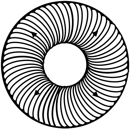
Consider a toroidal solenoid. This is a solenoid that is finite in length, and has had its axis bent such that the two open ends are closed upon each other, forming a classic doughnut (or bagel) shape. When we look at this device, from our perspective, the current is passing through the wires coming out of the page from the center of the toroid, and going into the page on the outside of the toroid (see the diagram below). use Ampère's law to find the field inside and outside the solenoid.

Solution

It's best to start by looking at a cross-section of the solenoid, slicing through the "bagel" parallel to the plane of the page . This shows wires on the inside with current coming out of the page, and wires on the outside with current going into the page.

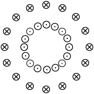
From symmetry, we can conclude that the magnetic field at any fixed distance from the center is the same magnitude, though the field strength may vary when that distance is changed. Also, symmetry demands that the field direction will have to be tangent to a circle in the plane of the page and concentric to the center of the toroid.

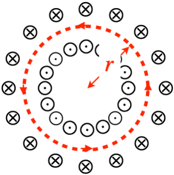
Constructing an Ampèrian circuit that is a circle in the plane of the page will then be parallel to whatever field is present anywhere, making the integral easy to do. If the radius of the circular path is \(r\), then:

\[\oint \overrightarrow B \cdot \overrightarrow {dl} = \oint B\;dl = B\oint dl = B\left(2\pi r\right) \nonumber\]

If we choose the circuit to be outside the toroid (or inside the doughnut hole), then the enclosed current is zero, which tells us that the magnetic field outside the toroid is zero. Like a straight solenoid, a toroidal solenoid confines the magnetic field to its interior. To get the field inside the solenoid, choose the radius of the circular path such that it is inside the solenoid:

This time the enclosed current is the total number of turns in the solenoid \(N\) multiplied by the current through the wire \(I\), giving us the field inside:

\[B\left(2\pi r\right) = \mu_o N I \;\;\;\Rightarrow\;\;\; B=\dfrac{\mu_o N I}{2\pi r} \nonumber\]

Notice that this differs from the field in a straight solenoid in two ways: First, the field is not uniform within the solenoid – it is stronger closer to the center than it is near the outside of the solenoid. And second, it is the total number of turns (which is now finite) rather than the turn density that determines the field strength. Interestingly, the turn density for the toroid can be adjusted to "turns per radian" rather than turns per meter. This "angular turn density" is simply \(\frac{N}{2\pi}\).

Local (Differential) Form of Ampère's Law

Just as with the case of Gauss’s law, we can use a theorem from vector calculus to convert Ampère’s law into local form. The name of the theorem in question is Stokes' theorem, and it states that for a vector field \(\overrightarrow B\left(\overrightarrow r\right) \):

\[\oint \overrightarrow B \cdot \overrightarrow {dl} = \int \left(\overrightarrow \nabla \times \overrightarrow B\right)\cdot d\overrightarrow A\;,\]

where the closed path borders the area over which the area integral is performed. If we now apply Ampère's law to this and note that the current that passes through the area equals the flux of the current density, we get:

\[\int \left(\overrightarrow \nabla \times \overrightarrow B\right)\cdot d\overrightarrow A = \mu_o I_{encl} = \mu_o \int \overrightarrow J \cdot d\overrightarrow A \;\;\;\Rightarrow\;\;\; \overrightarrow \nabla \times \overrightarrow B = \mu_o \overrightarrow J\]

As with the local form of Gauss's law, this provides us with a means for doing calculations that would otherwise be more difficult using the integral form.