
4.4: Sources of Magnetic Fields
- Page ID
- 21535

\( \newcommand{\vecs}[1]{\overset { \scriptstyle \rightharpoonup} {\mathbf{#1}} } \)
\( \newcommand{\vecd}[1]{\overset{-\!-\!\rightharpoonup}{\vphantom{a}\smash {#1}}} \)
\( \newcommand{\dsum}{\displaystyle\sum\limits} \)
\( \newcommand{\dint}{\displaystyle\int\limits} \)
\( \newcommand{\dlim}{\displaystyle\lim\limits} \)
\( \newcommand{\id}{\mathrm{id}}\) \( \newcommand{\Span}{\mathrm{span}}\)
( \newcommand{\kernel}{\mathrm{null}\,}\) \( \newcommand{\range}{\mathrm{range}\,}\)
\( \newcommand{\RealPart}{\mathrm{Re}}\) \( \newcommand{\ImaginaryPart}{\mathrm{Im}}\)
\( \newcommand{\Argument}{\mathrm{Arg}}\) \( \newcommand{\norm}[1]{\| #1 \|}\)
\( \newcommand{\inner}[2]{\langle #1, #2 \rangle}\)
\( \newcommand{\Span}{\mathrm{span}}\)
\( \newcommand{\id}{\mathrm{id}}\)
\( \newcommand{\Span}{\mathrm{span}}\)
\( \newcommand{\kernel}{\mathrm{null}\,}\)
\( \newcommand{\range}{\mathrm{range}\,}\)
\( \newcommand{\RealPart}{\mathrm{Re}}\)
\( \newcommand{\ImaginaryPart}{\mathrm{Im}}\)
\( \newcommand{\Argument}{\mathrm{Arg}}\)
\( \newcommand{\norm}[1]{\| #1 \|}\)
\( \newcommand{\inner}[2]{\langle #1, #2 \rangle}\)
\( \newcommand{\Span}{\mathrm{span}}\) \( \newcommand{\AA}{\unicode[.8,0]{x212B}}\)
\( \newcommand{\vectorA}[1]{\vec{#1}} % arrow\)
\( \newcommand{\vectorAt}[1]{\vec{\text{#1}}} % arrow\)
\( \newcommand{\vectorB}[1]{\overset { \scriptstyle \rightharpoonup} {\mathbf{#1}} } \)
\( \newcommand{\vectorC}[1]{\textbf{#1}} \)
\( \newcommand{\vectorD}[1]{\overrightarrow{#1}} \)
\( \newcommand{\vectorDt}[1]{\overrightarrow{\text{#1}}} \)
\( \newcommand{\vectE}[1]{\overset{-\!-\!\rightharpoonup}{\vphantom{a}\smash{\mathbf {#1}}}} \)
\( \newcommand{\vecs}[1]{\overset { \scriptstyle \rightharpoonup} {\mathbf{#1}} } \)
\(\newcommand{\longvect}{\overrightarrow}\)
\( \newcommand{\vecd}[1]{\overset{-\!-\!\rightharpoonup}{\vphantom{a}\smash {#1}}} \)
\(\newcommand{\avec}{\mathbf a}\) \(\newcommand{\bvec}{\mathbf b}\) \(\newcommand{\cvec}{\mathbf c}\) \(\newcommand{\dvec}{\mathbf d}\) \(\newcommand{\dtil}{\widetilde{\mathbf d}}\) \(\newcommand{\evec}{\mathbf e}\) \(\newcommand{\fvec}{\mathbf f}\) \(\newcommand{\nvec}{\mathbf n}\) \(\newcommand{\pvec}{\mathbf p}\) \(\newcommand{\qvec}{\mathbf q}\) \(\newcommand{\svec}{\mathbf s}\) \(\newcommand{\tvec}{\mathbf t}\) \(\newcommand{\uvec}{\mathbf u}\) \(\newcommand{\vvec}{\mathbf v}\) \(\newcommand{\wvec}{\mathbf w}\) \(\newcommand{\xvec}{\mathbf x}\) \(\newcommand{\yvec}{\mathbf y}\) \(\newcommand{\zvec}{\mathbf z}\) \(\newcommand{\rvec}{\mathbf r}\) \(\newcommand{\mvec}{\mathbf m}\) \(\newcommand{\zerovec}{\mathbf 0}\) \(\newcommand{\onevec}{\mathbf 1}\) \(\newcommand{\real}{\mathbb R}\) \(\newcommand{\twovec}[2]{\left[\begin{array}{r}#1 \\ #2 \end{array}\right]}\) \(\newcommand{\ctwovec}[2]{\left[\begin{array}{c}#1 \\ #2 \end{array}\right]}\) \(\newcommand{\threevec}[3]{\left[\begin{array}{r}#1 \\ #2 \\ #3 \end{array}\right]}\) \(\newcommand{\cthreevec}[3]{\left[\begin{array}{c}#1 \\ #2 \\ #3 \end{array}\right]}\) \(\newcommand{\fourvec}[4]{\left[\begin{array}{r}#1 \\ #2 \\ #3 \\ #4 \end{array}\right]}\) \(\newcommand{\cfourvec}[4]{\left[\begin{array}{c}#1 \\ #2 \\ #3 \\ #4 \end{array}\right]}\) \(\newcommand{\fivevec}[5]{\left[\begin{array}{r}#1 \\ #2 \\ #3 \\ #4 \\ #5 \\ \end{array}\right]}\) \(\newcommand{\cfivevec}[5]{\left[\begin{array}{c}#1 \\ #2 \\ #3 \\ #4 \\ #5 \\ \end{array}\right]}\) \(\newcommand{\mattwo}[4]{\left[\begin{array}{rr}#1 \amp #2 \\ #3 \amp #4 \\ \end{array}\right]}\) \(\newcommand{\laspan}[1]{\text{Span}\{#1\}}\) \(\newcommand{\bcal}{\cal B}\) \(\newcommand{\ccal}{\cal C}\) \(\newcommand{\scal}{\cal S}\) \(\newcommand{\wcal}{\cal W}\) \(\newcommand{\ecal}{\cal E}\) \(\newcommand{\coords}[2]{\left\{#1\right\}_{#2}}\) \(\newcommand{\gray}[1]{\color{gray}{#1}}\) \(\newcommand{\lgray}[1]{\color{lightgray}{#1}}\) \(\newcommand{\rank}{\operatorname{rank}}\) \(\newcommand{\row}{\text{Row}}\) \(\newcommand{\col}{\text{Col}}\) \(\renewcommand{\row}{\text{Row}}\) \(\newcommand{\nul}{\text{Nul}}\) \(\newcommand{\var}{\text{Var}}\) \(\newcommand{\corr}{\text{corr}}\) \(\newcommand{\len}[1]{\left|#1\right|}\) \(\newcommand{\bbar}{\overline{\bvec}}\) \(\newcommand{\bhat}{\widehat{\bvec}}\) \(\newcommand{\bperp}{\bvec^\perp}\) \(\newcommand{\xhat}{\widehat{\xvec}}\) \(\newcommand{\vhat}{\widehat{\vvec}}\) \(\newcommand{\uhat}{\widehat{\uvec}}\) \(\newcommand{\what}{\widehat{\wvec}}\) \(\newcommand{\Sighat}{\widehat{\Sigma}}\) \(\newcommand{\lt}{<}\) \(\newcommand{\gt}{>}\) \(\newcommand{\amp}{&}\) \(\definecolor{fillinmathshade}{gray}{0.9}\)Magnetic Field of a Long Straight Wire
We begin by computing the field of a long-straight wire that carries a current \(I\). Aside from the vectors, the procedure follows almost exactly the same path as the case of the electric field of a long line of charge.
Figure 4.4.1 – Calculating Magnetic Field of Long, Straight Wire
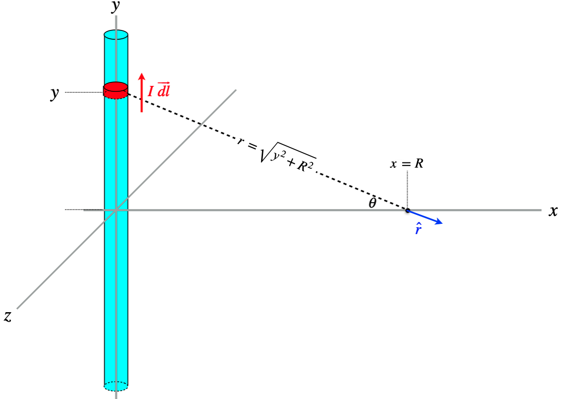
One of the key differences between computing magnetic fields and electric fields is that while we were able to use symmetry to help us solve for components of the electric field, in the case of the magnetic field, this is much harder to do, and is much safer to just get all the vectors right and trust vector math thereafter. We could have used this "trust the vector math" approach for the electric field as well, of course, but the necessity of using it in cases where cross-products are involved becomes quickly apparent.
Okay, we start by expressing all the relevant quantities in terms of our chosen coordinate system:
\[\begin{array}{l} \overrightarrow {dl} =dy\;\widehat j && \widehat r = \cos\theta\;\widehat i - \sin\theta\;\widehat j && \cos\theta = \dfrac{R}{\sqrt{y^2+R^2}} \end{array}\]
Next, write down Biot-Savart's law for the current element, and simplify:
\[\begin{array}{l} d\overrightarrow B && = \left(\dfrac{\mu_o}{4\pi}\right)\dfrac{I}{r^2}\overrightarrow {dl} \times \widehat r \\ &&= \left(\dfrac{\mu_oI}{4\pi}\right)\dfrac{dy}{y^2+R^2}\widehat j \times \left(\cos\theta\;\widehat i - \sin\theta\;\widehat j\right) \\ &&= \left(\dfrac{\mu_oI}{4\pi}\right)\dfrac{dy}{y^2+R^2} \left(\cos\theta\;\cancelto{-\widehat k}{\widehat j \times\widehat i} - \sin\theta\;\cancelto{-0}{\widehat j \times\widehat j}\right) \\ &&= \left(\dfrac{\mu_oI}{4\pi}\right)\dfrac{dy}{y^2+R^2}\left(\dfrac{R}{\sqrt{y^2+R^2}}\right)\left(-\widehat k\right) \\ &&= \left(\dfrac{\mu_oI\;R}{4\pi}\right)\dfrac{dy}{\left(y^2+R^2\right)^{\frac{3}{2}}}\left(-\widehat k\right)\end{array}\]
All that remains is to add up the contributions to the field from all the current elements, which means integrating this from \(y=-\infty\) to \(y=+\infty\):
\[\begin{array}{l} \overrightarrow B && = \left(-\widehat k\right)\left(\dfrac{\mu_oI\;R}{4\pi}\right) \int\limits_{-\infty}^{+\infty} \dfrac{dy}{\left(y^2+R^2\right)^{\frac{3}{2}}} \\ && = \left(-\widehat k\right)\left(\dfrac{\mu_oI\;R}{4\pi}\right) \left[\dfrac{1}{R^2}\;\dfrac{y}{\sqrt{y^2+R^2}}\right]_{-\infty}^{+\infty} \\ && = \left(-\widehat k\right)\left(\dfrac{\mu_oI}{4\pi R}\right)\left[2\right] \\ && = \left(\dfrac{\mu_oI}{2\pi R}\right)\left(-\widehat k\right) \end{array}\]
The resemblance the magnitude of this field bears to that of the electric field (Equation 1.5.2) is interesting, though not all that surprising, given that both fields weaken with distance from the source according to an inverse-square law. The direction of the magnetic field vector is tangent to a circle centered at the line of the current, and circles around the current line.
Figure 4.4.2 – Magnetic Field Circulates Around the Long, Straight Wire
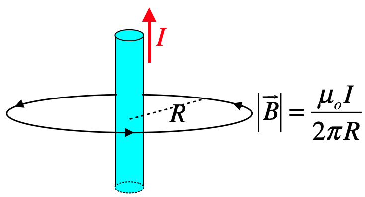
As with the electric field, the magnetic field obeys superposition, which means we can combine the result of this physical situation with others to get a net magnetic field. It is also worth noting that both the moving point charge and the long, straight wire yield magnetic fields whose line close back on themselves (form closed loops) – in nether case does a field emanate out of or into the source. There are no magnetic monopole fields.
Field of a Loop
Another useful field to know is that which points along the axis of a circular loop of current. The method is essentially the same as above, but the coordinate system used is different, which leads to a little bit more complicated vector manipulation.
Figure 4.4.3 – Calculating Magnetic Field on the Axis of a Circular Loop of Current
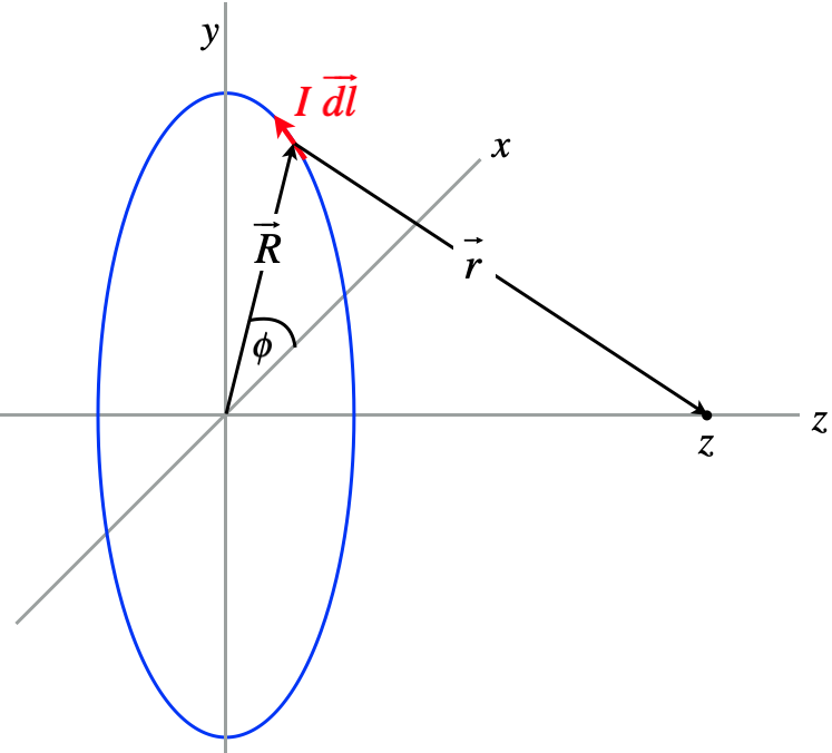
Again start by expressing quantities in terms of the coordinates we have set up. We can again write everything in terms of the \(ijk\) unit vectors, but this time we can do it a bit differently. First we have the magnitude of the segment of wire:
\[\left|\overrightarrow{dl}\right| =R\;d\phi\]
Next we note that tail-to-head vector addition gives:
\[\overrightarrow R + \overrightarrow r = z \widehat k\;\;\;\Rightarrow\;\;\; \overrightarrow r = - \overrightarrow R + z \widehat k\]
Biot-Savart's law gives:
\[d\overrightarrow B = \dfrac{\mu_o}{4\pi} \dfrac{I\overrightarrow{dl}\times\overrightarrow r}{r^3} \]
Before we can integrate, we have to resolve the vector products. Looking at the diagram, we can see that the current element \(\overrightarrow{dl}\), the position vector of the current element \(\overrightarrow R\), and the unit vector \(\widehat k\) are all mutually orthogonal, making \(\overrightarrow{dl} \times \overrightarrow R\) parallel to \(\widehat k\), and \(\overrightarrow{dl} \times \widehat k\) parallel to \(\overrightarrow R\). This allows us to use the right-hand rule to complete these products:
\[\overrightarrow{dl}\times\overrightarrow r=\overrightarrow{dl}\times\left(-\overrightarrow R + z\widehat k\right) = R\;dl\;\widehat k + z\;dl\;\widehat R\]
Putting this result into the integral and noting that magnitudes of the vectors \(\overrightarrow r\) and \(z\;\widehat k\) are constant in the integral, and satisfy \(r^2=R^2+z^2\), we get:
\[\overrightarrow B = \dfrac{\mu_oI}{4\pi} \int \dfrac{\overrightarrow{dl}\times\overrightarrow r}{r^3} = \dfrac{\mu_oI}{4\pi\left(R^2+z^2\right)^{\frac{3}{2}}}\int \left[R\;dl\;\widehat k +z\;dl\;\widehat R\right]\]
While the magnitude of \(\overrightarrow R\) doesn't change over the integral, its direction does change, so we have to write the unit vector \(\widehat R\) in terms of the coordinates to do the integral of the second term. Let's do each integral separately. The first is straightforward, since the integral of just \(dl\) is simply the circumference of the circle:
\[\begin{array}{l} \dfrac{\mu_oIR}{4\pi\left(R^2+z^2\right)^{\frac{3}{2}}}\widehat k\int dl = \dfrac{\mu_oIR^2}{2\left(R^2+z^2\right)^{\frac{3}{2}}}\widehat k \\ \dfrac{\mu_oIz}{4\pi\left(R^2+z^2\right)^{\frac{3}{2}}}\int dl \widehat R = \dfrac{\mu_oIz}{4\pi\left(R^2+z^2\right)^{\frac{3}{2}}}\int \limits_0^{2\pi} R\;d\phi \left(\cos\phi\;\widehat i + \sin\phi\;\widehat j\right)=0\end{array}\]
The second integral just ends up vanishing, giving the result for a magnetic field along the axis of a loop of radius \(R\) a distance \(z\) from the plane of the loop:
\[B = \dfrac{\mu_oIR^2}{2\left(R^2+z^2\right)^{\frac{3}{2}}}\]
If we are only interested in the field at the center of the loop, we plug in \(z=0\) to get the simple result:
\[B = \dfrac{\mu_oI}{2R}\]
The direction of \(\widehat k\) shows us yet another shortcut for using the right-hand-rule for the field along the axis (and only along the axis!) of a loop: Curl the fingers of the right hand such that they trace the circulation of the current around the loop, and the thumb points the direction of the field.
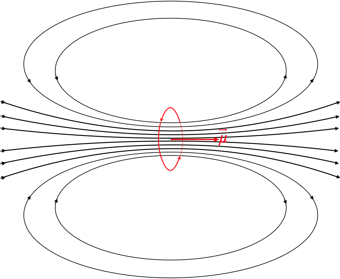
We have already talked about a loop as a magnetic dipole which interacts with fields that are present, and here (as in the case of the electric dipole), we see that the dipole also emits a field, and this field – like the electric dipole field – gets weaker as the inverse cube of the distance (which in this case is measured by \(z\)). Also, like the electric dipole, the field along its axis points in the direction of the dipole moment:
Figure 4.4.4 – Magnetic Dipole Field of a Loop
Field of a Solenoid
It is possible to stack lots of individual dipoles on top of each other to create a long tube called a solenoid. Such a device consists of a number of turns in the coil \(N\), and a length \(L\), resulting in what will be the critical measure, the turn density:
Figure 4.4.5 – A Solenoid
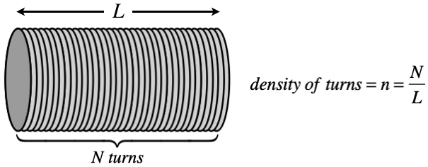
How do we compute the field for such an object? Well, first of all, we need to specify what field we want. Like the loop, we will only look on the axis. But we will also simplify it further by assuming we are looking at a point on the axis inside the solenoid far from the ends (so essentially it has an infinite length, though the turn density is of course finite).
We treat this as a collection of an infinite number of loops. If we pick an origin (which we can place anywhere along the infinite axis), then we have the field at that point by a loop at a position \(z\) on the axis is given by Equation 4.4.10. Then we need to add up the field contributions at the origin due to all of the loops. The problem is, there is not a loop at every point along the \(z\)-axis. With a turn density of \(n\), the number of turns in a tiny slice \(dz\) would be \(n\;dz\) The total current in that slice would then be this number multiplied by the current through the wound wire (which we will call \(I\)):
\[\text{current in a } dz \text{ slice located at } z = I\;n\;dz\]
Plugging this into Equation 4.4.10 for the current, gives the tiny contribution to the field by the slice, and adding them all up gives the field. We are not given the radius of the solenoid, but we will call it \(R\), and we'll see that it isn't relevant!
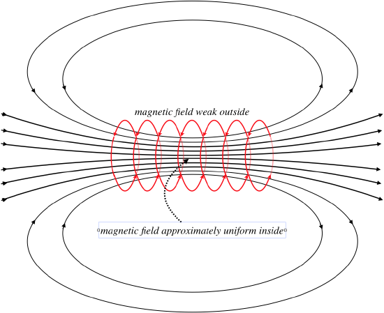
There are a few particularly interesting aspects of the fields of solenoids, which are not immediately evident from this solution, but which we will state without proof (for now – we have another tool to use later that makes this easier):
- The field within the solenoid doesn’t change much (it is pretty much uniform). This basically comes from the fact – as we found here – that the field on the axis doesn't depend upon the radius of the solenoid.
- The field just outside the solenoid (on its side, not the end) is very weak (basically it is zero).
- The field looks just like that of a bar magnet, but it can be turned on and off by switching the current on or off.
Figure 4.4.6 – Solenoid Magnetic Field
Digression: Electromagnets
Solenoids have lots of practical uses, a common one being something known as an “electromagnet.” For example, junk yards use these to move large chunks of scrap metal. Obviously the ability to cut the current to turn off the magnetic field is key here. If the crane used a permanent magnet, it wouldn’t be able to let go of the crushed car. Another application is for fire doors. Imagine large doors held open in hallways of a building with electromagnets, and if a fire breaks out, the power is cut and the doors close, hopefully slowing the spread of the fire. Gates where you are “buzzed-in” are held shut by a latch that is released with the activation of an electromagnet that draws the latch back with a magnetic field.
Magnetic Materials
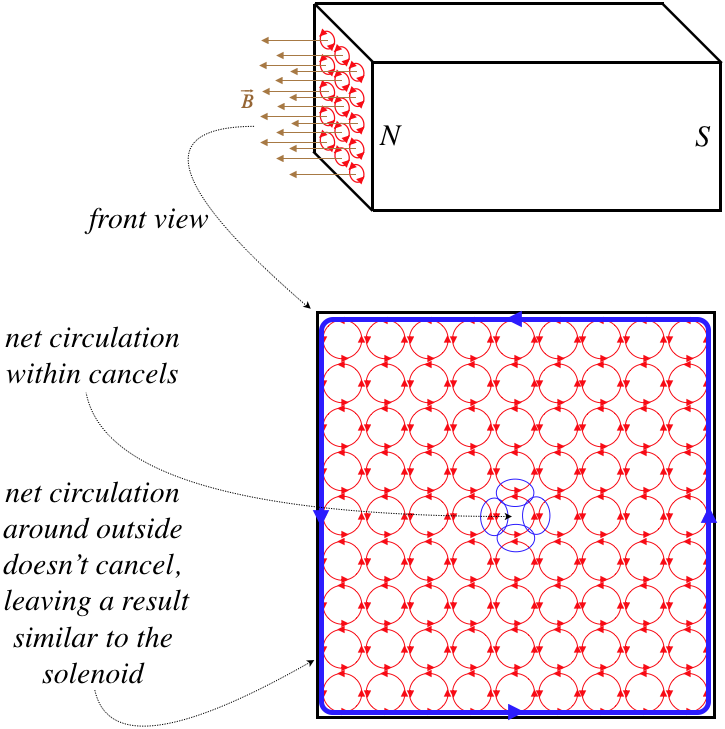
At last we can discuss elements of magnetism that we have been aware of since we were young kids – the properties and behavior of bar magnets. As with any phenomenon that requires an understanding of what is going on at a microscopic level, magnetism inside of materials like bar magnets is very complicated. We’ll look at a greatly-simplified version of it here, but keep in mind that a fuller understanding can only be achieved through quantum theory.
We now know that there are no “magnetic particles” comprising a bar magnet – its magnetic field can only be created by moving charges. But unlike an electromagnet, bar magnets are not plugged into some emf source, so where does the moving charge come from? The atoms that comprise the material of course include lots of charges, and these charges are moving in manners that resemble magnetic dipoles – electrons are orbiting nuclei in more-or-less circular loops, and electrons also have a quantum-mechanical property called “spin” that gives them their own magnetic moments as well.
We will not concern ourselves too much with the specific source of the magnetic moments of these particles, but we will instead just focus on the fact that each particle has its own magnetic moment. In the case of a bar magnet, these dipoles tend to be permanently aligned. This property is called ferromagnetism. Only a few materials have this property: iron (thus “ferro”), nickel, cobalt, many of their alloys, and some of the rare earth metals. [Technically, these alignments occur in chunks, called “domains,” within the magnet, and the degree to which the magnet is magnetized is determined by how much certain domains “swallow-up” others, creating more broadly-coordinated alignments of dipoles.]
Figure 4.4.7 – Dipoles in a Bar Magnet
It should be clear how two bar magnets attract each other. One is a magnetic field source, and the other is a magnetic dipole that experiences the non-uniform field of the other. The field diverges as it emerges from one magnet, and the dipole of the other magnet, if the poles are aligned, reacts by feeling a force in the direction where the field gets stronger, following the mechanism depicted in Figure 4.2.6.
But this doesn’t explain why a magnet sticks to a refrigerator when the refrigerator metal is not itself magnetized. The answer is that some metals, while their particle dipole moments are not permanently aligned, have the property that their particles are free to rotate their magnetic moments. When an external field is applied, their particles then align, making them magnetized. When the field is removed, the random alignments return. This property is known as paramagnetism.
A few general comments to close this subject:
- Ferromagnetism relies primarily upon the spin source of magnetic moment, and very little on the orbital source, while paramagnetism relies upon both.
- Ferromagnetic materials remain magnetized after a strong applied magnetic field aligns the domains, which remain aligned thanks to anomalies in the crystal structure which “snag” the domains and hold them in an aligned orientation.
- Ferromagnets can be demagnetized (“degaussed”) by relieving these snags. This is most easily done by raising the temperature to a critical temperature known as the Curie temperature, at which magnetic domain "snags” are no longer possible and the substance has zero ferromagnetism. Other methods for degaussing include applying rapidly-changing magnetic fields (which “shake” the domains into random orientations) and pounding on the magnet so that vibrations cause the domains to un-snag.