1.3: Interference Effects

Standing Waves

Sound can create a variety of interference effects, like any other wave. Among those interference effects are standing waves. These are formed in precisely the way described for strings in Physics 9B, with two traveling waves reflecting back-and-forth between two endpoints. In the case of sound in a gas, it isn't immediately clear what constitutes "fixed" and "free" endpoints, since sound waves in gas do not involve particles of media that can ever be held in place. We have to broaden our notion of what it means to have a fixed boundary to mean simply that whatever physical quantity plays the role of "displacement" for a wave is unchanging. In the case of sound, this would mean pressure or density. We will see in a moment how this can be.

We are used to talking about one-dimensional standing waves, so it is fair to ask how this can be set up for sound in a gas. If a region of the gas has a pressure higher than the ambient pressure, the gas will naturally expand into the lower-pressure region, so to create a 1-dimensional standing sound wave, we must set up circumstances so that the compressed regions doesn't expand into all three dimensions. We can do this by producing the sound within a hollow pipe. The fixed or free boundary conditions at the ends of the pipe then depend upon whether the end of the pipe is open or closed, but which case is fixed, and which is free?

Let's look first at a closed end. When a compression propagates its way toward a closed end, the means for the compression to restore itself to equilibrium is restricted – it can't continue forward. The compression grows even greater than the amplitude of the wave, just as the displacement of a string at the point of reflection from a free end grows above the amplitude (see Figure 1.5.5 in the 9B textbook). So in fact a closed end of a hollow pipe represents a "free" end for a standing sound wave.

The open end is quite different. In fact, it does not behave like an end at all, but rather like a transition point. We know this is true if we follow the energy – a sound wave headed for an open end will transmit energy out of that open end, as the compressions and rarefactions are transmitted to the region of the gas outside the pipe. So why would there be any reflection back into the pipe at all? As in the case of going from slow-to-fast or fast-to-slow medium, the mathematics of the boundary interaction is beyond this course, but the result is the same. The obvious objection here is that the speed of the wave within the air in the pipe is no different from the speed of sound outside the pipe. This is true, and in fact it requires a bit of a revision to that observation. Perhaps a better way of describing the reflection/transmission phenomenon is to say that there is at least partial reflection whenever the wave equation governing the wave changes. One way for the wave equation to change is for the wave velocity to change. Another is for the wave to go from being confined to one dimension to three dimensions. This is exactly what happens when the sound in a pipe emerges from an open end.

We know that waves in three-dimensions spread the energy very fast, causing the amplitude to drop-off in proportion to the distance. It is therefore not a bad approximation to claim that at the open end (or slightly beyond it) is at a fixed pressure/density (the ambient pressure/density). This means that if we are forced to choose, the open end of the pipe to a good approximation behaves like a fixed end, and the sound wave that reflects back into the pipe is phase-shifted.

From these considerations, we now know that standing sound waves in a pipe create pressure antinodes at closed ends, and pressure nodes at open ends. Armed with this information, we can use all the same machinery regarding standing waves that we learned in Physics 9B. What is interesting about the case of sound is how this can be used to create tones in organ pipes and wind instruments. These devices make use of two special aspects of standing waves in pipes. The first we have already mentioned – an open end allows for some transmission of sound waves, which means that we can hear the tone produced without having to crawl inside the pipe. The second has to do do with the idea of resonance.

Digression: Resonance

Resonance is a very important concept in many fields of physics, and we unfortunately don't have time to cover it in great detail here, though it will come up again in both Physics 9C and 9D. The main idea is that if vibrating systems interact with each other, the amount of energy that can be transmitted from one to the other is largely dependent upon how closely the "natural frequencies" (think of masses on springs with frequencies that look like \(\omega=\sqrt{\frac{k}{m}}\)) of those systems match. If the frequencies are a good match, then the superposition of the displacements of the two systems leads to constructive interference. If they don't match, then the displacements don't synchronize, and there is very little overall constructive interference. A good analogy is pushing a child on a swing. If you give them a push forward every time they reach the peak of their backswing, then the frequency of your pushes matches the natural frequency of the swing, and energy is transmitted to the swing. If, however, you were to push with a different frequency, then some of the pushes would add energy to the swing, but many others would push the swing forward as it is coming backward, taking energy away from the swing.

If we get air moving near the end of a pipe, like when we blow into a flute, the result is turbulent flow. This adds energy to the system, but the waves created come in a wide variety of frequencies. All of these sound waves travel the length of the pipe, partially reflecting and transmitting when they get there. But as we have seen in our study of standing waves, only those waves that have one of the harmonic wavelengths will exhibit the constructive interference required for a standing wave. Those waves that do have the right frequency exhibit resonance, building energy for the standing wave at that frequency. The result is that of the many sound waves that escape the pipe, those at a resonant frequency of the pipe (determined by its length) have by far the most energy, and are the only sounds heard. It turns out that by far most of the energy goes to the fundamental harmonic, though overtones can also often be heard. To modulate the frequency of the sound that escapes therefore becomes a matter of changing the length of the pipe. An organ designates a pipe for every key on the keyboard; a slide trombone allows the player to physically expand the length of the pipe; valves and holes in other wind instruments also serve this same purpose. Note also that all of these instruments rely upon the turbulent flow to provide the spectrum of sound waves, whether it is through a vibrating reed, vibrating lips, or air forced across an open end. (Note: Air forced into an open end does not induce much turbulence compared to air forced across the opening.)

Lastly, it should be noted that to produce a sustained tone, one must continually add energy. This is because energy is always exiting the pipe via the transmitted wave. The rate at which energy is added equals the rate of energy escaping via sound waves, while the energy in the standing wave within the pipe remains constant.

Example \(\PageIndex{1}\)

A string is plucked above a pipe that is open at one end, and the fundamental harmonic tone is heard coming from the pipe. If the closed end of the pipe is now opened, how must the tension of the string be change in order to excite the new fundamental harmonic?

Solution

Open ends of pipes act as fixed points (nodes) for standing sound waves. The fundamental harmonic of the pipe with one end closed fits one quarter of a wave between the ends of the pipe (node to first antinode), while the first harmonic with both ends open fits a half-wavelength (node to node). Therefore opening a closed end shrinks the wavelength of the fundamental harmonic by a factor of 2. The speed of the sound wave is unchanged, so its fundamental harmonic frequency rises a factor of 2. The standing sound wave is being driven by (i.e. is getting energy from) the standing wave in the string, so their frequencies must match for this resonance to occur, which means that when the end of the pipe is opened, the string's standing wave frequency must also rise by a factor of 2. The string has not changed length, so the only other way to change its frequency is to change the speed of the traveling wave on the string. To double the speed of the string wave (and therefore double the frequency), the tension must be quadrupled, since the wave speed on the string is proportional to the square root of the tension, and the linear density of the string cannot be changed.

Beats

Up to now, all of our cases of interference involve waves that have identical frequencies. But a very interesting phenomenon emerges when two sound waves interfere that have slightly different frequencies (actually any two different frequencies will do, but the phenomenon is easier to detect when the frequencies are within 1 or 2 hertz, for reasons we will see). We'll start with another over-simplified diagram like those we have used above. This time, the two waves emerging from the speakers will have different frequencies, and therefore different wavelengths (though for simplicity, we will assume they have the same amplitude).

Figure 1.3.4 – Superposing Two Sound Waves of Different Frequencies

The diagram is of course a snapshot at a moment in time. If, at this moment in time, a listener is positioned at the left vertical line, then the superposition of the two waves results in constructive interference, which means that the sound heard is loud. If, on the other hand, someone is positioned at the right vertical line, then destructive interference results in silence. But now suppose that one remains at the right vertical line for a short time after this snapshot is taken. Both waves are traveling at the same speed (they are both in the same medium), so the rarefactions that coincide at the left vertical line will soon be at the right vertical line. That is, a person listening at the right vertical line will, at one moment, hear silence, and then a short time later, a loud tone. This pattern will in fact repeat itself with regularity, and this pulsing of the sound is referred to as beats.

The math that governs this phenomenon results from a straightforward application of trigonometric identities. We start with a wave function for each wave. As we are talking about sound for which the "displacement" is pressure, we will represent the wave function with the variable \(P\left(x,t\right)\). Note we are also keeping things simple by staying in one dimension:

\[P_1\left(x,t\right) = P_o\cos\left(\frac{2\pi}{\lambda_1}x-\frac{2\pi}{T_1}t+\phi_1\right)\;,\;\;\;\;\;P_2\left(x,t\right) = P_o\cos\left(\frac{2\pi}{\lambda_2}x-\frac{2\pi}{T_2}t+\phi_2\right)\]

We are interested in what is happening to the sound at a single point in space (i.e. we want to show it gets it gets louder and softer), and any point will do, so for simplicity we'll choose the origin, \(x=0\). This reduces our two functions to:

\[P_1\left(t\right) = P_o\cos\left(-\frac{2\pi}{T_1}t+\phi_1\right)\;,\;\;\;\;\;P_2\left(t\right) = P_o\cos\left(-\frac{2\pi}{T_2}t+\phi_2\right)\]

These functions are oscillating with different frequencies, so they are out-of-sync. We can choose a position and time when one of these waves is at a maximum, and define these as \(x=0\) and \(t=0\), respectively.  For this wave, we have essentially set its phase constant \(\phi\) equal to zero. There is no guarantee that the other wave will also be at a maximum at this place and time, so we can't arbitrarily set the other phase constant equal to zero as well.  If they do have a relative phase that is non-zero, then it turns out that the combined sound will not be as loud as if they waves were in phase, but the general features described below remain the same.  To simplify the math, we will therefore just look at the simple case where the waves are in phase, and set \(\phi_1=\phi_2=0\). With the phase constants equal to zero, we now have a simple pair of functions to work with (note that we can drop the minus signs on the times, since \(\cos\left(x\right)=\cos\left(-x\right)\)). Superposing these and replacing the periods with frequencies gives:

\[P_{tot}\left(t\right)=P_1\left(t\right)+P_2\left(t\right)=P_o\cos\left(2\pi f_1 t\right)+P_o\cos\left(2\pi f_2 t\right)\]

Now apply a trigonometric identity:

\[\cos X + \cos Y = 2\cos\left(\dfrac{X-Y}{2}\right)\cos\left(\dfrac{X+Y}{2}\right) \\ \Rightarrow\;\;\; P_{tot}\left(t\right)=2P_o\cos\left[2\pi\left(\dfrac{f_1-f_2}{2}\right)t\right]\cos\left[2\pi\left(\dfrac{f_1+f_2}{2}\right)t\right]\]

This looks like a complicated mess, but there is a reasonable way to interpret it. If we identify the second cosine function as the variation of the pressure that defines the time portion of the sound wave (often referred to as the carrier wave), the tone produced has a frequency that is the average of the two individual frequencies. The first cosine function can then be combined with \(2P_o\), and together they can be treated as a time-dependent amplitude. The amplitude is directly related to the intensity, which is a measure of the loudness of the sound, so a harmonically-oscillating amplitude would manifest itself as regularly-spaced increases and decreases in volume (beats). It's a bit easier to see how this works with a diagram.

Figure 1.3.5 – Graph of Pressure vs. Time at a Fixed Point Exhibiting Beats

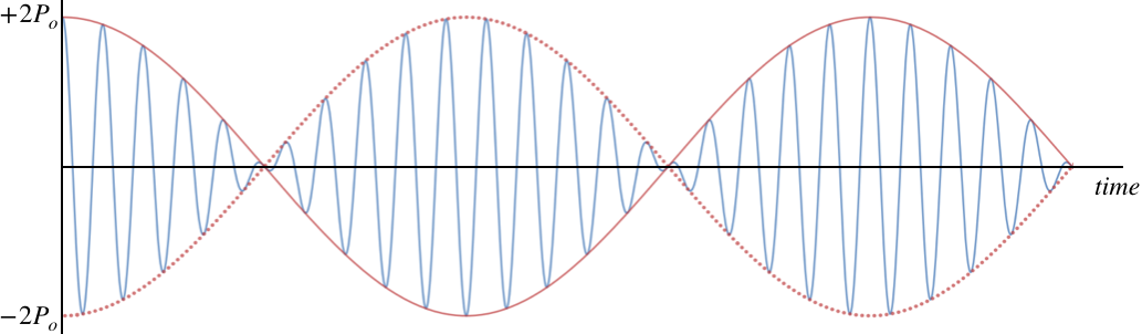
The blue function shown represents the fluctuations in pressure (at position \(x=0\) as a function of time as the sound wave passes through that point. Notice that the peaks have varying heights, reflecting the time-varying amplitude. The red "envelope" function traces just the amplitude of the wave. The intensity is proportional to the square of the amplitude, so the sound is loud everywhere that a red bump occurs, and silence is heard when the red function crosses the axis.

Alert

The volume of the sound doesn't drop to zero every time the blue graph crosses the axis! That is simply when the pressure happens to be passing through the equilibrium point, and there is still energy in a wave when the displacement of the medium passes through the equilibrium point (in the form of kinetic energy of the medium). But when the amplitude of oscillations goes to zero, the energy is zero, and in the case of sound, this means silence.

We can ask how frequently the beats occur. A beat occurs every time a bump in the red graph occurs. Notice it doesn't matter whether the bump is up or down in the red cosine function, since the intensity is the square of the amplitude. Therefore there are two beats are heard for every full period of the red cosine function; one for the bump at the peak, and one for the bump at the trough. This means that the frequency of beats is twice the frequency of the red cosine function:

\[f_{beat} = 2\left(\dfrac{f_1-f_2}{2}\right) = f_1-f_2\]

[Note: We have assumed that \(f_1\) is the greater of the two frequencies, as negative frequencies have no meaning. One can remove this assumption by defining beat frequency in terms of the absolute value.] We can measure the time spans between peaks for the blue function. This is the period of the carrier wave, which we have already stated is the average of the frequencies of the two sound waves:

\[f_{carrier} = \dfrac{f_1+f_2}{2}\]

We only really hear the beats clearly when the two individual frequencies are close together – if there is too great of a difference, then the beat frequency is very high, and the beats come too frequently. In this case it’s impossible for the human ear to tell when one beat begins and the other ends. In that case, it sounds to the human ear more like a mixture of two sounds – one at the average frequency and one at the much lower "beat frequency."

Example \(\PageIndex{3}\)

A standing wave of sound persists within a hollow pipe that is open at both ends. A bug within the pipe walks along its length at a speed of \(4.0\frac{cm}{s}\). As it does so it passes through nodes and antinodes of the standing wave, hearing the tone get alternately loud and silent, with the time between moments of silence equaling 2.0s. From what we have learned about standing waves, we can compute the frequency of the tone. The distance between the nodes is one-half wavelength of the traveling sound wave, and based on the ant's speed and the time between nodes, we can determine this distance. Then with the wavelength and the speed of sound, we get the frequency:

\[\text{distance between nodes}=v_{bug}t=\frac{\lambda}{2}\;\;\;\Rightarrow\;\;\;\lambda=2\left(4.0\frac{cm}{s}\right)\left(2.0s\right)=16cm\;\;\;\Rightarrow\;\;\;f=\frac{v}{\lambda}=\dfrac{344\frac{m}{s}}{0.16m}=2150Hz\nonumber\]

When asked about the experience, the bug claimed it had no idea that it was walking through loud and silent regions. It described the experience as hearing periodic "beats" every 2.0 seconds in the tone. Re-derive the frequency of the sound from the perspective of the bug.

Solution

This problem is challenging because it's not immediately clear how beats can occur, when beats require two sound waves of different frequencies. There are two sound waves here – one reflected by each end of the pipe – but they both have the same frequency... or do they? They have the same frequency from our perspective, but not from the bug's! The bug is moving toward one end of the pipe and away from the other, so one of the waves is doppler-shifted to a higher frequency, and the other wave is doppler-shifted to a lower frequency. These waves of different frequencies interfere to provide beats from the ant's perspective. So now that we see how this makes sense, we need to do some math. Both doppler shifts involve a stationary source (the ends of the pipe) and a moving receiver (the bug):

\[f_1=\left(\dfrac{v+v_{ant}}{v}\right)f\;\;\;\;\;\;f_2=\left(\dfrac{v-v_{ant}}{v}\right)f\nonumber\]

The frequency \(f_1\) is what is heard by the ant from the wave coming from in front of it, and \(f_2\) is the frequency of the sound coming from behind it, and \(f\) is the frequency of the sound from the perspective of the stationary ends of the pipes (i.e. the frequency of the standing wave). The beat frequency heard by the ant is simply the difference of these two frequencies, so:

\[f_{beat} = f_1-f_2 = \left(\dfrac{v+v_{ant}}{v}\right)f - \left(\dfrac{v-v_{ant}}{v}\right)f = 2\dfrac{v_{ant}}{v}f\nonumber\]

We know that the bug hears silence every 2.0 seconds, so the beat frequency is \(0.50Hz\). Plugging this, the speed of the ant, and the speed of sound into this equation gives:

\[f=\dfrac{v}{2v_{ant}}f_{beat} = \dfrac{344\frac{m}{s}}{2\left(0.040\frac{m}{s}\right)}\left(0.5Hz\right)=2150Hz\nonumber\]

While we have worked this out for some specific numbers, it is of course true in general. If the bug was moving faster, then the pulses at the antinodes would come more frequently. From the bug's perspective the doppler shifts would greater separate the two individual sound frequencies, leading to a higher difference and faster beat frequency, and this identically equals the rate of passing through antinodes.