Module 1 - Summary

Summary Notes Module 1

Postulates of Ray Optics

• #1. Light travels in the form of rays
• #2. An optical medium is characterized by a refractive index, \( n \geq 1 \). The refractive index provides a measure of the speed of the light in that medium (\( v \)): \( n = \frac{c}{v} \) where \( c = 3 \times 10^8 \, \text{m/s} \).
• #3. The optical path length is the optical distance between two points: \[ \text{OPL} = \int_A^B n(x, y, z) \, ds, \] where \( ds \) is the differential distance between both points. If the medium is homogeneous, \( n(x, y, z) = \text{constant} \), the optical path length is equal to \( \text{OPL} = n \Delta \), where \( \Delta \) is the distance between points \( A \) and \( B \).
• #4. Fermat’s Principle: light traveling between two points follows a path in which the derivative of the OPL is zero. Therefore, the OPL is at a maximum, minimum, or a point of inflection.

Rules of propagation

• #1. In a homogeneous medium (i.e., \( n(x, y, z) = \text{constant} \)), the path of minimum distance between two points is a straight line. In other words, light travels in straight lines.
• #2. Law of reflection: the angle of reflection is the same as the angle of incidence.
• #3. The angle of refraction depends on the angle of incidence by Snell’s law: \[ n_1 \sin \theta_1 = n_2 \sin \theta_2. \]

Mirrors

• Planar mirror
• Paraboloidal mirror (i.e., focusing mirror) – all parallel rays to its optical axis are focused in the same point \( F \) (i.e., there is a focal spot). The distance defined by \( F \) and the mirror’s vertex \( P \) is the focal length.
• Elliptical mirror (i.e., image mirror) – all rays emitted from one focus are imaged onto the other focus. The distance traveled by the light between both focal spots is always the same regardless of the path. The elliptical mirror is defined by 2 focal spots.
• Spherical mirror – parallel rays are reflected to its optical axis at different positions. However, rays traveling close to its axis are approximately focused onto the same point \( F \), with the distance equal to half the distance to its center. In other words, the focal length \( f = - \frac{R}{2} \), where \( R \) is the radius of curvature. Note that convex mirrors have negative focal length \( f = - \frac{R}{2} \), and concave mirrors have positive focal length, \( f = \frac{R}{2} \).

Convex Mirror

Concave Mirror

Note the following sign convention: \( d_0, d_i < 0 \) means points to the right side of the mirror (i.e., virtual) and \( d_0, d_i > 0 \) are related to points to the left side of the mirror (i.e., real).

Ray Tracing in Mirrors

Convex Mirror

Concave Mirror

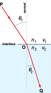
Planar Boundaries – a planar interface that separates two media of constant refractive index.

\[ n_1 \sin \theta_1 = n_2 \sin \theta_2 \] \[ n_1 \theta_1 \approx n_2 \theta_2 \quad \text{if} \quad \theta_1, \theta_2 \ll 1. \]

• #1. \( n_1 > n_2 \) then \( \theta_1 < \theta_2 \) – refracted rays away from the boundary.
• #2. \( n_1 < n_2 \) then \( \theta_1 > \theta_2 \) – refracted rays towards the boundary.
• #3. \( n_1 < n_2 \) and \( \theta_2 = 90^\circ \) – Phenomenon of Total Internal Reflection. \[ n_1 \sin \theta_1 = n_2 \sin \theta_2 = n_2 \sin(90^\circ) = n_2 \quad \Rightarrow \quad \sin \theta_1 = \frac{n_2}{n_1} \quad \Rightarrow \quad \theta_{1,c} = \sin^{-1} \left( \frac{n_2}{n_1} \right). \]

If the incidence angle is higher than the critical angle \( \theta_1 > \theta_{1,c} \), Snell’s law cannot be satisfied (i.e., \( \sin \theta_2 > 1 \)), so refraction does not occur and the incident ray is reflected (no refraction!). The phenomenon of total internal refraction occurs in fiber optics.

Lenses – two spherical surfaces of radii \( R_1 \) and \( R_2 \)

• Lens’ maker equation: \[ \frac{1}{f} = \frac{n - n_s}{n_s} \left( \frac{1}{R_1} - \frac{1}{R_2} \right) \] where \( f \) is the lens’ focal length, \( n \) is the lens’ refractive index, \( n_s \) is the refractive index of the surrounding media, and \( R_1 \) and \( R_2 \) are the radii of curvature of the first and second surfaces, respectively.
  • \( f > 0 \) is a converging lens and \( f < 0 \) is a diverging lens.
• Type of lenses (TIP: the name is associated with the outside shape):
  • Biconvex: \( R_1 > 0 \) and \( R_2 < 0 \)
  • Biconcave: \( R_1 < 0 \) and \( R_2 > 0 \)
  • Plano-convex: \( R_1 > 0 \) and \( R_2 = \infty \)
  • Plano-concave: \( R_1 = \infty \) and \( R_2 > 0 \)
• Imaging equations: \[ \frac{1}{d_0} + \frac{1}{d_i} = \frac{1}{f}, \quad y_i = - \frac{d_i}{d_0} y_0 \]
• Ray tracing

Converging Lens

Diverging Lens

Matrix Optics

Input \( \begin{bmatrix} A & B \\ C & D \end{bmatrix} \) Output

\[ \begin{pmatrix} y_2 \\ \theta_2 \end{pmatrix} = \begin{bmatrix} A & B \\ C & D \end{bmatrix} \begin{pmatrix} y_1 \\ \theta_1 \end{pmatrix} \]

\[ y_2 = A y_1 + B \theta_1, \quad \theta_2 = C y_1 + D \theta_1. \]

Matrix Element Value	Output Height or Angle	Consequence of the resultant system
\( A = 0\)	\( y_2 = B \theta_1 \)	Focusing system
\( B = 0\)	\( y_2 = A y_1 \)	Imaging system where \(A\) is the lateral magnification
\( C = 0\)	\( \theta_2 = D \theta_1 \)	Parallel rays remain parallel
\( D = 0\)	\(\theta_2 = C y_1 \)	Rays emerging from a point source are parallel after the system

Examples of ABCD Matrices

• Free propagation of a distance \( d \): \( \begin{bmatrix} 1 & d \\ 0 & 1 \end{bmatrix} \)
• Lens of focal length \( f \): \( \begin{bmatrix} 1 & 0 \\ -\frac{1}{f} & 1 \end{bmatrix} \) where \( f > 0 \) for converging lenses and \( f < 0 \) for diverging lenses.

Cascade of Matrices – an optical system composed of \( N \) matrices:

Input \( \begin{bmatrix} M_1 & M_2 & \dots & M_N \end{bmatrix}\) Output

\[ \begin{pmatrix} y_2 \\ \theta_2 \end{pmatrix} = \begin{bmatrix} M_T \end{bmatrix} \begin{pmatrix} y_1 \\ \theta_1 \end{pmatrix} \]

where \( M_T = M_N M_{N-1} \dots M_2 M_1 \).