Module 4 - Summary

Summary Notes Module 4

• Any amplitude distribution can be expressed as a sum of plane waves, i.e., \( \exp[j 2\pi (u x + v y)]. \) Compared to the mathematical expression of a plane wave in Module 2, \( \exp[j(k_x x + k_y y)], \) then \( k_x = 2\pi u = \frac{2\pi}{\lambda} \sin \theta_x \) and \( k_y = 2\pi v = \frac{2\pi}{\lambda} \sin \theta_y \). This means that the angle of the plane waves along the x- and y-direction can be estimated by \( \theta_x = \sin^{-1}(\lambda u) \quad \text{and} \quad \theta_y = \sin^{-1}(\lambda v). \)

• An imaging system must be a linear shift-invariant system. Consider that an imaging system is represented by a \( \mathbf{S} \) operator.

A system is linear if the output is equal to the sum of the individual outputs.

A system is shift-invariant if the output of a displaced input signal is the same function but displaced by the same amount.

Only when the optical system is linear space-invariant (LSI), the output signal, \( g(x, y) \), can be expressed as the two-dimensional (2D) convolution (\( \otimes_2 \)) between the input signal, \( f(x, y) \), and the impulse response of the system, \( h(x, y) \): \[ g(x, y) = f(x, y) \otimes_2 h(x, y). \]

In the Fourier domain, the spectrum of the output signal, \( G(u, v) \), is the product between the spectrum of the input signal, \( F(u, v) \), and the optical transfer function, \( H(u, v) \): \[ G(u, v) = F(u, v) H(u, v). \] This means that the transfer function \( H(u, v) \) is the 2D Fourier transform of the impulse response, \( h(x, y) \): \[ H(u, v) = \text{FT}[h(x, y)]. \]

• Free-space propagator under the Fresnel approximation

\[ h(x, y) = \frac{e^{j k z}}{j \lambda z} \exp\left[ j \frac{k}{2z}(x^2 + y^2) \right], \] and \[ H(u, v) = \frac{e^{j k z}}{j \lambda z} \exp\left[-j \pi \lambda z (u^2 + v^2)\right]. \]

Condition of the Fresnel region: \[ N_F \frac{\theta_m^2}{4} \ll 1, \] where \( N_F = \frac{a^2}{\lambda z} \) is the Fresnel number and \( \theta_m = \frac{a}{z} \) is the maximum aperture angle.

• Free-space propagator under the Fraunhofer approximation (\( z \gg \))

\[ g(x, y) = f(x, y) \otimes_2 h(x, y) = F \left( \frac{x}{\lambda z}, \frac{y}{\lambda z} \right) = F \left( \frac{x}{M}, \frac{y}{M} \right), \] where \( M \) is the magnification factor.

For \( z \gg \), the amplitude distribution (also known as the diffraction pattern) of an object transmittance \( f(x, y) \) is a scaled version of its Fourier Transform under Fraunhofer approximation.

Condition of the Fraunhofer region: \[ z \gg \frac{b_{\text{input}}^2}{\lambda} \quad \text{and} \quad z \gg \frac{a_{\text{output}}^2}{\lambda}, \] where \( b_{\text{input}} \) is the maximum lateral extent in the input plane and \( a_{\text{output}} \) is the maximum lateral extent in the output plane.

• Converging and diverging (i.e., optical) lenses make Fourier transforms.

Consider a converging lens. If an object with amplitude transmittance \( t(x, y) \) is placed at the front focal plane of a lens (i.e., the distance between the object/input and lens planes is equal to the lens’ focal length, \( f \)), a scaled replica of the Fourier transform of the object transmittance is found at its back focal plane: \[ T \left( \frac{x}{\lambda f}, \frac{y}{\lambda f} \right). \]

• Calculation of the complex amplitude distribution of an arbitrary optical system with an input transmittance \( t(x, y) \). The arbitrary optical system is represented by its ABCD matrix.

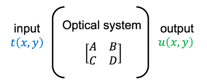
If \( B = 0 \), the complex amplitude distribution at the output plane is the product of a quadratic phase wavefront and a scaled replica of the object transmittance: \[ u(x, y) = e^{j k L_0 / A} \exp \left[ j \frac{k C}{2A} (x^2 + y^2) \right] t \left( \frac{x}{A}, \frac{y}{A} \right), \] where \( L_0 \) is the geometrical distance between the input and output planes and \( k = \frac{2\pi}{\lambda} \) is the wave number.

Else, if \( B \neq 0 \), the complex amplitude distribution at the output plane becomes: \[ u(x, y) = \frac{e^{j k L_0}}{j \lambda B} \exp \left[ j \frac{k D}{2B} (x^2 + y^2) \right] \int_{-\infty}^{\infty} t(x_0, y_0) \exp \left[ j \frac{k A}{2B} (x_0^2 + y_0^2) \right] \exp \left[ -j \frac{2\pi}{\lambda B} (x x_0 + y y_0) \right] \, dx_0 \, dy_0. \]

• 4f imaging system if both lenses have the same focal length

• 4f imaging system if both lenses have different focal lengths

• Spatial filtering in a 4f imaging system by inserting a pupil with transmittance \( p(x, y) \) at the Fourier plane of a 4f system. The pupil filters out some object frequencies.

Thus, the complex amplitude at the image plane (i.e., back focal plane of the \( L_2 \) lens) is: \[ u(x, y) = \frac{1}{M^2} t \left( \frac{x}{M}, \frac{y}{M} \right) \otimes_2 P \left( \frac{x}{\lambda f_2}, \frac{y}{\lambda f_2} \right) = \frac{1}{M^2} t \left( \frac{x}{M}, \frac{y}{M} \right) \otimes_2 h(x, y), \] where \( M = - \frac{f_2}{f_1} \) is the lateral magnification, \( \otimes_2 \) is the 2D convolution operator, and \( P(u, v) \) is the 2D Fourier transform of the pupil transmittance. Based on the equation, the impulse response of the 4f imaging system is a scaled replica of the pupil’s Fourier transform, \( h(x, y) = P \left( \frac{x}{\lambda f_2}, \frac{y}{\lambda f_2} \right) \). Therefore, the transfer function is a scaled replica of the pupil’s transmittance: \[ H(u, v) = \text{FT}[h(x, y)] = p \left( -\frac{\lambda f_2 u}{f_1}, -\frac{\lambda f_2 v}{f_1} \right). \]