Error Analysis

1 - Introduction

"To err is human; to describe the error properly is sublime."
-- Cliff Swartz, Physics Today 37 (1999), 388.

As you may know, most fields in the physical sciences are bifurcated into two branches: theory and experiment. In general, the theoretical aspect is taught in lectures, tutorials and by doing problems, while the experimental aspect is learned in the laboratory.

The way these two branches handle numerical data are significantly different. For example, here is a problem from the end of a chapter of a well-known first year University physics textbook:

A particle falling under the influence of gravity is subject to a constant acceleration g of 9.8 m/s². If …

Although this fragment is perfectly acceptable for doing problems, i.e. for learning theoretical Physics, in an experimental situation it is incomplete. Does it mean that the acceleration is closer to 9.8 than to 9.9 or 9.7? Does it mean that the acceleration is closer to 9.80000 than to 9.80001 or 9.79999? Often the answer depends on the context. If a carpenter says a length is "just 8 inches" that probably means the length is closer to 8 0/16 in. than to 8 1/16 in. or 7 15/16 in. If a machinist says a length is "just 200 millimeters" that probably means it is closer to 200.00 mm than to 200.05 mm or 199.95 mm.

We all know that the acceleration due to gravity varies from place to place on the earth's surface. It also varies with the height above the surface, and gravity meters capable of measuring the variation from the floor to a tabletop are readily available. Further, any physical measurement such as of g can only be determined by means of an experiment, and since a perfect experimental apparatus does not exist it is impossible even in principle to ever know g perfectly. Thus in an experimental context we must say something like:

A 5 g ball bearing falling under the influence of gravity in Room 126 of McLennan Physical Laboratories of the University of Toronto on March 13, 1995 at a distance of 1.0 ± 0.1 m above the floor was measured to be subject to a constant acceleration of 9.81 ± 0.03 m/s².

This series of documents and exercises is intended to discuss how an experimentalist in the physical sciences determines the errors in a measurement, i.e. the numbers that appear to the right of the ± symbols in the above statement. The level is appropriate for beginning University students in the sciences.

We should emphasis right now that a correct experiment is one that has been correctly performed. Thus:

The error in an experimentally measured quantity is never found by comparing it to some number found in a book or web page.

Also, although we will be exploring mathematical and statistical procedures that are used to determine the error in an experimentally measured quantity, as you will see these are often just "rules of thumb" and sometimes a good experimentalist uses his or her intuition and common sense to simply guess.

Although these notes are delivered via the web, many people find that reading the type of material discussed here is more effective on paper than on a computer screen. If you are one of these people you may wish to print out these notes and read them in hardcopy.

However, because of different browsers and choices of default fonts printing this version of the document which you are now reading may not "layout" very cleanly on the page . Thus another version of this document has been prepared in the Portable Document Format (pdf) with page breaks controlled for a better layout. Using pdf files requires that you have the Acrobat Reader software installed, which is available free from http://www.adobe.com.

The file size of the pdf version is 290k and the hardcopy will be 37 pages. It will appear in a separate window. You may access the pdf version of this document here.

The pdf version will produce better hardcopy, but the version you are now reading will be easier to use and read in your browser

2 - Motivation

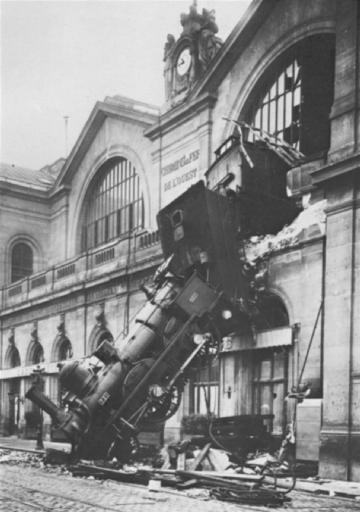A lack of understanding of basic error analysis has led some very bright scientists to make some incredible blunders. Here we give only three examples of many.

Example 1 - Cold Fusion

In 1989 two University of Utah researchers, Stanley Pons and Martin Fleischmann, announced that they had produced nuclear fusion with a laboratory bench apparatus consisting of palladium rods immersed in a bath of deuterium, or heavy water. The scientists said their device emitted neutrons and gamma rays, which are certain signatures of nuclear, as opposed to chemical, reactions.

This announcement caused a huge reaction in the popular press, and there were many statements being made that this was the beginning of unlimited free energy for the world.

The claim turned out to be wrong: cold fusion in this form does not exist. Amongst other mistakes, Pons and Fleischman neglected to do the simple error analysis on their results which would have shown that they had not achieved cold fusion in their lab.

You may learn more about this sad episode in the history of Physics by clicking here.

Example 2 - High Fiber Diets

In the early 1970's researchers reported that a diet that was high in fiber reduced the incidence of polyps forming in the colon. These polyps are a pre-cursor to cancer.

As a consequence of these studies, many people have since been eating as much fiber as they could possibly get down their gullet.

In January 2000 a massive study published in the New England Journal of Medicine indicated that fiber in the diet has no effect on the incidence of polyps.

The problem with the earlier studies is that the limited number of people in the samples meant that the results were statistically insignificant. Put another way, the error bars of the measurements were so large that the 2 samples, with and without high fiber diets, gave cancer rates that were numerically different but were the same within errors.

Note the word statistically in the previous paragraph: it indicates correctly that some knowledge of statistics will be necessary in our study of error analysis.

Example 3 - A Very Silly Fit

Two of the very highest prestige scientific journals in the world are Nature and Science. Here is a figure and caption from an article published by David W. Roubik in Science 201 (1978), 1030.

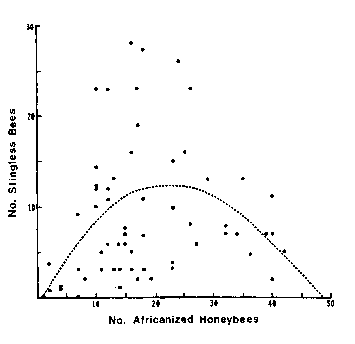
The dashed line is a quadratic polynomial (given by y = -0.516 + 1.08x - 0.23x²) which gave the best fit to the points.

It seems fairly clear that this "best fit to the points" in fact has no relationship whatsoever to what the data actually look like. In fact, some think the data look more like a duck, with the beak in the upper-left and pointing to the left. You may access a little Flash animation about this I put together on a quiet afternoon by clicking on the button to the right; it will appear in a separate window and has a file size of 17k.

3 - Backgammon 101

As mentioned in the previous section, the topic of error analysis requires some knowledge of statistics. Here we begin our very simple study.

Although we used the word "simple" in the previous sentence, perhaps surprisingly it was not until the sixteenth century that correct ideas about probability began to be formed

For example, an annuity is an investment in which a bank receives some amount of money from a customer and in return pays a fixed amount of money per year back to the customer. If a fairly young customer wants to buy an annuity from the bank, the probability is that he or she will live longer than an older customer would. Thus the bank will probably end up making more payments to a young customer than an older one. Note that the argument is statistical: it is possible for the young customer to get killed by a runaway bus just after buying the annuity so the bank doesn't have to make any payments.

Thus the probabilities say that if the bank wishes to make a profit, for younger customers it should either charge more for the annuity or pay back less per year than for older customers.

The lack of the concept of what today is called "simple statistics" prior to the sixteenth century meant, for example, that when banks in England began selling annuities, it never occurred to them that the price to the customer should be related to his/her age. This ignorance actually caused some banks to go bankrupt.

Similarly, although people have been gambling with dice and related apparatus at least as early as 3500 BCE, it was not until the mid-sixteenth century that Cardano discovered the statistics of dice that we will discuss below.

For an honest die with an honest roll, each of the six faces are equally likely to be facing up after the throw. For a pair of dice, then, there are 6 × 6 = 36 equally likely combinations.

Of these 36 combinations there is only one, 1-1 ("snake eyes"), whose sum is 2. Thus the probability of rolling a two with a pair of honest dice is 1/36 = 3%.

There are exactly two combinations, 1-2 and 2-1, whose sum is three. Thus the probability of rolling a three is 2/36 = 6%.

The following table summarises all of the possible combinations:

Probabilities for honest dice

Sum	Combinations	Number	Probability
2	1-1	1	1/36=3%
3	1-2, 2-1	2	2/36=6%
4	1-3, 3-1, 2-2	3	3/36=8%
5	2-3, 3-2, 1-4, 4-1	4	4/36=11%
6	2-4, 4-2, 1-5, 5-1, 3-3	5	5/36=14%
7	3-4, 4-3, 2-5, 5-2, 1-6, 6-1	6	6/36=17%
8	3-5, 5-3, 2-6, 6-2, 4-4	5	5/36=14%
9	3-6, 6-3, 4-5, 5-4	4	4/36=11%
10	4-6, 6-4, 5-5	3	3/36=8%
11	5-6, 6-5	2	2/36=6%
12	6-6	1	1/36=3%

A histogram is a convenient way to display numerical results. You have probably seen histograms of grade distributions on a test. If we roll a pair of dice 36 times and the results exactly match the above theoretical prediction, then a histogram of those results would look like the following:

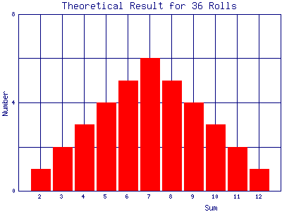
Exercise 3.1: roll a pair of honest dice 36 times, recording each result. Make a histogram of the results. How do your results compare to the theoretical prediction?

It is extremely unlikely that the result of Exercise 3.1 matched the theory very well. This is, of course, because 36 repeated trials is not a very large number in this context. Clicking on the following button will open a new browser window that will give you an opportunity to explore what the phrase "large number" means. There you will also find some questions to be answered.

One of the lessons that you may have learned from Exercise 3.2 is that even for a large number of repeated throws the result almost never exactly matches the theoretical prediction. Exercise 3.3 explores this further.

After completing Exercise 3.3, you may wish to think about the fact that, except for the first, all of the combinations of number of rolls times number of repetitions gave a total of 36,000 total rolls. This means that if we had a single set of 36,000 rolls of a pair of dice we could get different width curves of the same shape just by partitioning the data in different ways.

Question 3.1. What is the probability of rolling a seven 10 times in a row?

Question 3.2. Amazingly, you have rolled a seven 9 times in a row. What is the probability that you will get a seven on the next roll?

Backgammon, like poker, is a game of skill disguised as a game of chance: the most skillful player wins in the long run. In backgammon the most skilled player is the one who best understands the material of this section. If both players are equally ignorant of this material, which one wins the game is, literally, a crap shoot.

4 - Bell Shaped Curves

"Whenever a large sample of chaotic elements are taken in hand … an unsuspected and most beautiful form of regularity proves to have been latent all along."
--- Francis Galton, 19^th century

We saw in Exercise 3.3 that bell shaped curves arise when we repeat rolls of dice and look at, say, the fraction of sevens. Other examples of where such curves commonly arise include:

Grade distributions for a class. This example is the Fall marks from a first year Physics laboratory at the University of Toronto. The "sample size" is 845 students. The small excess for very low marks is probably from students who have dropped the laboratory but still appear in the mark database.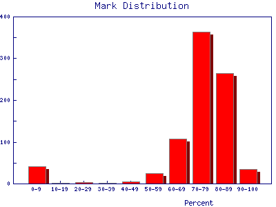
Heights of people. This is data for 928 people born of 205 pairs of parents. The data were taken in England by Galton in 1886.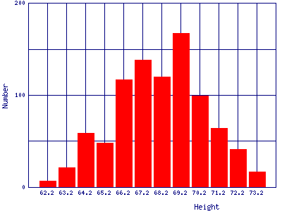
Radioactive decay. Here are data of the number counts in one second from a Cesium-37 radioactive source. The measurements were repeated 100 times.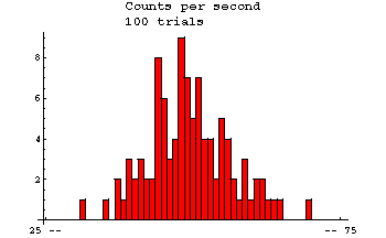

Data that are shaped like this are often called normal distributions. The most common mathematical formula used to describe them is called a Gaussian, although it was discovered 100 years before Gauss by de Moivre. The formula is:

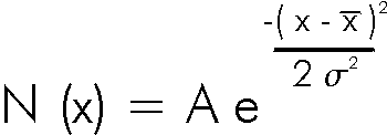
which looks like:

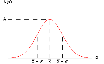
The symbol A is called the maximum amplitude.

The symbol is called the mean or average.

The symbol is called the standard deviation of the distribution. Statisticians often call the square of the standard deviation, ², the variance; we will not use that name. Note that is a measure of the width of the curve: a larger means a wider curve. ( is the lower case Greek letter sigma.)

The value of N(x) when x = + or - is about 0.6065 × A, as you can easily show.

Soon it will be important to note that 68% of the area under the curve of a Gaussian lies between the mean minus the standard deviation and the mean plus the standard deviation. Similarly, 95% of the curve is between the mean minus twice the standard deviation and the mean plus twice the standard deviation.

In the quotation at the beginning of this section, Galton refers to chaotic elements. In 1874 Galton invented a device to illustrate the meaning of "chaotic." It is called a quincunx and allows a bead to drop through an array of pins stuck in a board. The pins are equally spaced in a number of rows and when the bead hits a pin it is equally likely to fall to the left or the right. It then lands on a pin in the next row where the process is repeated. After passing through all rows it is collected in a slot at the bottom. After a large number of beads have dropped, the distribution is Gaussian.

A simulation of a quincunx is available here.

Question 4.1. In Exercise 3.3 you were asked to find a numerical way of measuring the width of the distributions. One commonly used method is to find the "full width at half the maximum" (FWHM). To find this you determine where the number of data is one-half of the value of the maximum, i.e. where N(x) = A/2. There will be two such points for a bell shaped curve. Then the FWHM is the difference between the right hand side value and the left hand side value of x. For a Gaussian distribution what is the mathematical relationship between the FWHM and the standard deviation?

Question 4.2. You have a large dataset that is normally distributed. If you choose one data point at random from the dataset, what is the probability that it will lie within one standard deviation of the mean?

In everyday usage the word chaotic, which has been used above, means utter confusion and disorder. In the past 40 years, a somewhat different meaning to the word has been formed in the sciences. Just for interest, you may learn more about scientifically chaotic systems here. A difference in the meaning of words in everyday versus scientific contexts is common; examples include energy and momentum.

5 - Using the Gaussian

In the previous section we saw examples of data that are distributed at least approximately like a Gaussian. Here we again show the data taken by Galton on heights, this time with a Gaussian curve superimposed on it:

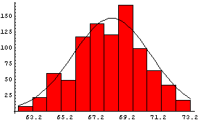
The amplitude of the curve is 146.4, the mean is 68.2, and the standard deviation is 2.49.

Of course, the data do not perfectly match the curve because "only" 928 people were measured.

If we could increase the sample size to infinity, we might expect the data would perfectly match the curve. However there are problems with this:

• For data like the height data, we can not even in principle increase the sample size to infinity since there are not an infinite number of people in the world.
• For data like the radioactive decays which we also looked at in the previous section, it would take an infinite amount of time to repeat the measurements an infinite number of times.
• For many types of data, such as the height data, clearly the assumption of a normal distribution is only an approximation. For example, the Gaussian only approaches zero asymptotically at ± infinity. Thus if the height data is truly Gaussian we could expect to find some people with negative heights, which is clearly impossible! Nonetheless, we will often find that treating data as if it were normally distributed is a useful approximation.

In the previous section we also looked at a distribution of laboratory marks. It is shown again to the right. We imagine that we will ignore the small excess of students with very low marks, since almost all of them have actually dropped the laboratory. We typically would like to know the mean of the other marks so we may know how good the average student is. We would also like to know the standard deviation so we may know how diverse the students are in their laboratory ability.

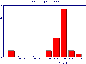
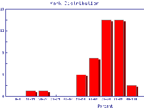
We also may wish to find out the same information for the marks of individual Teaching Assistants to judge student ability and also perhaps to see if the TAs are all marking consistently. Here are the mark distributions for four of the Teaching Assistants in the laboratory.

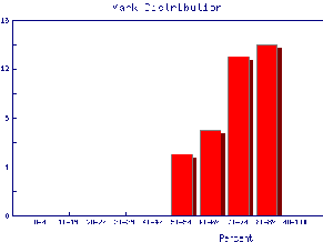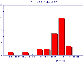For each of these five mark distributions, it is fairly clear that the limited sample sizes mean that we can only estimate the mean; we will give the estimated mean the symbol . It is calculated by adding up all the individual marks X_i and dividing by the number of marks N.

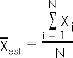
Similarly, we can only estimate the standard deviation, which we will give the symbol . The statisticians tell us that the best estimate of the standard deviation is:

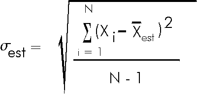
Note that the above equation indicates that can not be calculated if N is one. This is perfectly reasonable: if you have only taken one measurement there is no way to estimate the spread of values you would get if you repeated the measurement a few times.

The quantity N - 1 is called the number of degrees of freedom.

The point we have been making about estimated versus true values of the mean and standard deviation needs to be emphasized:

For data which are normally distributed, the true value of the mean and the true value of the standard deviation may only be found if there are an infinite number of data points.

In the previous section we looked at some data on the number of decays in one second from a radioactive source. Here we shall use this sort of data to explore the estimated standard deviation.

In Question 4.2, you hopefully answered that there is a 68% chance that any measurement of a sample taken at random will be within one standard deviation of the mean. Usually the mean is what we wish to know and each individual measurement almost certainly differs from the true value of the mean by some error. But there is a 68% chance that any single measurement lies with one standard deviation of this true value of the mean. Thus it is reasonable to say that:

The standard deviation is the error in each individual measurement of the sample.

The error in a quantity is usually indicated by a , so the above statement may be written as:

\[\Delta x_i=\sigma\]

This error is often called statistical. We shall see other types of errors later.

Often what we really want to know is the error in the estimated mean. However, we will need to learn some more about error analysis before we can discuss this topic.

Question 5.1. Listed here are twenty measurements of the time for a stone to fall from a window to the ground, in hundredths of a second.

63	58	74	78	70	64	75	82	68	29
76	62	72	88	65	81	79	77	66	76

Compute the estimated mean and the estimated standard deviation of the twenty measurements.

In Exercise 5.1 you saw that the estimated standard deviation was different for each trial with a fixed number of repeated measurements. In fact, if you make a histogram of a large number of trials it will show that these estimated standard deviations are normally distributed. It can be shown that the standard deviation of this distribution of estimated standard deviations, which is the error in each value of the estimated standard deviation, is:

Since the estimated standard deviation is the error in each individual measurement, the above formula is the error in the error!

6 - The Reading Error

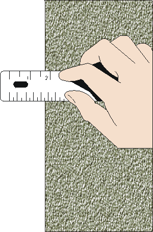In the previous section we saw that when we repeat measurements of some quantity in which random statistical factors lead to a spread in the values from one trial to the next, it is reasonable to set the error in each individual measurement equal to the standard deviation of the sample.

Here we discuss another error that arises when we do a direct measurement of some quantity: the reading error.

For example, to the right we show a measurement of the position of the left hand side of some object with a ruler. The result appears to be just a bit less than 1.75 inches.

We shall assume that the ruler is perfectly constructed. This assumption is discussed further in Section 12.

To determine the reading error in this measurement we have to answer the question: what is the minimum and maximum values that the position could have for which we will not see any difference? There is no fixed rule that will allow us to answer this question. Instead we must use our intuition and common sense.

Could the value actually be as large as 1.75? Perhaps, but almost certainly no larger. Could the value be as small as 1.70? Very unlikely. How about 1.73? Perhaps, but probably no smaller. Thus a reasonable estimate of the reading error of this measurement might be ± 0.01 inches. Then we would state that the position is 1.74 ± 0.01 inches.

For your eyes and computer monitor with which you are looking at the above measurement, you may wish to instead associate a reading error of 0.02 inches with the position; this is also a reasonable number. A reading error of 0.03 inches, though, is probably too pessimistic. And a reading error much less than 0.01 is probably too optimistic.

To the right we show the same measurement, but with two differences. First it is smaller. Second the person doing the measurement needs to clean their glasses. It seems fairly obvious that the reading error for this measurement will be larger than for the previous one.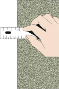

We assume that the reading error indicates a spread in repeated measurements, just like the standard deviation discussed in the previous section. However, here natural human biases means that each repeated measurement should be done by a different person. So if we get a collection of objective observers together to look at the first measurement above, we expect most but perhaps not all observers will report a value between 1.73 and 1.75 inches. (Of course, in real life seldom if ever do we actually get a collection of observers together so that we may determine the reading error of a simple measurement.)

Note that there is often a trade-off when assigning a reading error such as above. On the one hand we want the error to be as small as possible, indicating a precise measurement. However we also want to insure that measured value probably lies within errors of the "true" value of the quantity, which means we don't want the error to be too small.

Exercise 6.1. Choose your textbook or some other hardcover book and measure its thickness. What is the reading error in this measurement? Repeat the measurement a few times at different places on the book. What is the estimated standard deviation of your measurements?

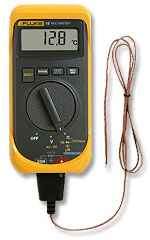For a measurement with an instrument with a digital readout, the reading error is "± one-half of the last digit."

We illustrate with a digital thermometer shown to the right.

The phrase "± one-half of the last digit" above is the language commonly used in manufacturer's specification sheets of their instruments. It can be slightly misleading. It does not mean one half of the value of the last digit, which for this example is 0.4. It means one-half of the power of ten represented in the last digit. Here, the last digit represents values of a tenth of a degree, so the reading error is 1/2 x 0.1 = 0.05.

This is saying that the value is closer to 12.8 than to 12.7 or 12.9. It assumes that the engineer who designed the instrument has made it round measurements correctly in the display.

Finally, then we would write the temperature as 12.80 ± 0.05 ^oC.

One sometimes sees statements that the reading error of an analog instrument such as a meter stick is something like ± one-half of the smallest scale marking. These and similar statements are wrong! The reading error of such an analog instrument can only be determined by the person reading the instrument, and can sometimes be different for different people.

7 - The Precision

In Sections 5 and 6 we saw two different specifications for the error in a directly measured quantity: the standard deviation and the reading error. Both are indicators of a spread in the values of repeated measurements. They both are describing the precision of the measurement.

The word precision is another example of an everyday word with a specific scientific definition. As we shall discuss later, in science precision does not mean the same thing as accuracy.

In any case, we now have two different numbers specifying the error in a directly measured quantity. But what is the error in the quantity?

The answer is both. But fortunately it is almost always the case that one of the two is much larger than the other, and in this case we choose the larger to be the error.

In Exercise 6.1 you measured the thickness of a hardcover book. Unless the book has been physically abused the standard deviation of your measurements was probably negligible and might even have been zero. Thus the error in your measurement is just the reading error.

In other cases, such as the number of radioactive decays in one second that we looked at in Sections 4 and 5, the reading error of the digital Geiger counter is ± 0.5 counts, which is negligible compared to the standard deviation. Thus here the error in each measurement is the standard deviation.

Often just thinking for a moment in advance about a measurement will tell you whether repeating it will be likely to show a spread of values not accounted for by the reading error. This in turn will tell you whether you need to bother repeating it at all.

If you don't know in advance whether or not you need to repeat a measurement you can usually find out by repeating it three or four times. If repeated measurements are called for, we will discuss in Section 10 how many repetitions is ideal.

8 - Significant Figures

Imagine we have some sample of 10 data points which we assume are normally distributed. The estimated standard deviation is numerically equal to 0.987654321, which is larger than the reading error for these measurements. (By "numerically" we mean that is what the calculator read when we computed the standard deviation.) Since the estimated standard deviation is larger than the reading error, it will be the error in the value of each of the data points.

As mentioned at the end of Section 5, when a sample has N data points the expected uncertainty in the estimated standard deviation is:

For this data, the error is numerically equal to 0.232792356, which is 23% of the value of the estimated standard deviation. This relatively high percentage is another way of expressing what you saw in Exercise 5.1, where even 50 repeated trials of the number of radioactive decays in one second was not a "large number" for data which have a significant spread.

What these numbers are saying is that we think the actual value of the standard deviation is probably greater than 0.987654321 - 0.232792356 = 0.704861965, and is probably less than 0.987654321 + 0.232792356 = 1.220446677. A moment's thought about this should convince you that many of the digits in the estimated standard deviation have no significance.

In fact, the value of the estimated standard deviation is something like: 0.99 ± 0.23 or maybe even 1.0 ± 0.2. Certainly 0.988 ± 0.233 has more digits in both the value and its error than are actually significant.

Examining the above formula for the error in the estimated standard deviation indicates that even if one repeats a measurement 50 times, the error in the estimated standard deviation is about 10% of its value. Put another way, even for N equal to 50 the estimated standard deviation has at most only two digits that have any meaning.

Imagine one of the data points has a numerical value of 12.3456789. Then if we take the estimated standard deviation to be 0.99, then the data point has a value of 12.35 ± 0.99, i.e. probably between 11.36 and 13.34. It would be wrong to say 12.345 ± 0.99, since the '5' has no meaning. It would also be wrong to say 12.35 ± 0.987, since the '7' similarly has no meaning. These examples illustrate a general conclusion:

For experimental data the error in a quantity defines how many figures are significant.

In the case where the reading error is larger than the estimated standard deviation, the reading error will be the error in each individual measurement. However as we saw in the previous section, the reading error is little more than a guess made by the experimenter. I do not believe that people can guess to more than one significant figure. Thus a reading error almost by definition has one and only one significant figure, and that number determines the significant figures in the value itself.

Above we saw that even if one repeats a measurement 50 times the standard deviation has at most two significant figures. And now we have seen that the reading error certainly does not have more than two significant figures. So in general:

In simple cases errors are specified to one or at most two digits.

Question 8.1. Express the following quantities to the correct number of significant figures:

(a) 29.625 ± 2.345
(b) 74 ± 7.136
(c) 84.26351 ± 3

9 - Propagation of Errors of Precision

Often we have two or more measured quantities that we combine arithmetically to get some result. Examples include dividing a distance by a time to get a speed, or adding two lengths to get a total length. Now that we have learned how to determine the error in the directly measured quantities we need to learn how these errors propagate to an error in the result.

We assume that the two directly measured quantities are X and Y, with errors X and Y respectively.

The measurements X and Y must be independent of each other.

The fractional error is the value of the error divided by the value of the quantity: X / X. The fractional error multiplied by 100 is the percentage error. Everything is this section assumes that the error is "small" compared to the value itself, i.e. that the fractional error is much less than one.

For many situations, we can find the error in the result Z using three simple rules:

Rule 1

If:

or:

then:

In words, this says that the error in the result of an addition or subtraction is the square root of the sum of the squares of the errors in the quantities being added or subtracted. This mathematical procedure, also used in Pythagoras' theorem about right triangles, is called quadrature.

Rule 2

If:

or:

then:

In this case also the errors are combined in quadrature, but this time it is the fractional errors, i.e. the error in the quantity divided by the value of the quantity, that are combined. Sometimes the fractional error is called the relative error.

The above form emphasises the similarity with Rule 1. However, in order to calculate the value of Z you would use the following form:

Rule 3

If:

then:

or equivalently:

For the square of a quantity, X², you might reason that this is just X times X and use Rule 2. This is wrong because Rules 1 and 2 are only for when the two quantities being combined, X and Y, are independent of each other. Here there is only one measurement of one quantity.

Question 9.1. Does the first form of Rule 3 look familiar to you? What does it remind you of? (Hint: change the delta's to d's.)

Question 9.2. A student measures three lengths a, b and c in cm and a time t in seconds:

a = 50 ± 4
b = 20 ± 3
c = 70 ± 3
t = 2.1 ± 0.1

Calculate a + b, a + b + c, a / t, and (a + c) / t.

Question 9.3. Calculate (1.23 ± 0.03) + . ( is the irrational number 3.14159265…)

Question 9.4. Calculate (1.23 ± 0.03) × .

Exercise 9.1. In Exercise 6.1 you measured the thickness of a hardcover book. What is the volume of that book? What is the error in that estimated volume?

You may have noticed a useful property of quadrature while doing the above questions. Say one quantity has an error of 2 and the other quantity has an error of 1. Then the error in the combination is the square root of 4 + 1 = 5, which to one significant figure is just 2. Thus if any error is equal to or less than one half of some other error, it may be ignored in all error calculations. This applies for both direct errors such as used in Rule 1 and for fractional or relative errors such as in Rule 2.

Thus in many situations you do not have to do any error calculations at all if you take a look at the data and its errors first.

The remainder of this section discusses material that may be somewhat advanced for people without a sufficient background in calculus.

The three rules above handle most simple cases. Sometimes, though, life is not so simple. The general case is where Z = f(X,Y). For Rule 1 the function f is addition or subtraction, while for Rule 2 it is multiplication or division. Regardless of what f is, the error in Z is given by:

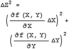
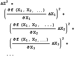
If f is a function of three or more variables, X₁, X₂, X₃, … , then:

---

The above formula is also used to find the errors for transcendental functions. For example if:

Z = ln(X)

then since the function f is only of one variable we replace the partial derivatives by a full one and:

Similarly, if:

Z = sin(X)

then:

Note that in the above example X must be in radian measure.

10 - The Error in the Mean

We have seen that when the data have errors of precision we may only estimate the value of the mean. We are now ready to find the error in this estimate of the mean.

Recall that to calculate the estimated mean we use:

Each individual measurement X_i has the same error, X, which is usually the estimated standard deviation.

To calculate the error in the numerator of the above equation, we use Rule 1 from Section 9 to write:

In words, we are combining N quantities X in quadrature, whose result is the square root of N times X.

When we divide the numerator by the denominator N, Rule 2 tells us how to propagate those errors. The denominator has an error of zero, and we have just calculated the error in the numerator. Applying Rule 2, then, gives:

In words, the error in the estimated mean is equal to the error in each individual measurement X divided by the square root of the number of times the measurement was repeated. Sometimes is called the standard error of the mean.

Here is an example. We repeat the measurement of some quantity 4 times and get:

Result
1.50
1.61
1.39
1.48

The estimated mean of these measurements is numerically 1.4950000 and the estimated standard deviation is numerically 0.0903696 (by numerically we mean the number that is displayed by the calculator). Thus the error in the estimated mean is 0.0903696 divided by the square root of the number of repeated measurements, the square root of 4, which is numerically 0.0451848. So we get:

Value = 1.495 ± 0.045

or:

Value = 1.50 ± 0.04

The fact that the error in the estimated mean goes down as we repeat the measurements is exactly what should happen. If the error did not go down as N increases there is no point in repeating the measurements at all since we are not learning anything about X_est, i.e. we are not reducing its error.

In Section 7 we promised to discuss how many times one should repeat a measurement. Although one answer is as many times as possible, unless the data collection is automated and/or you have lots of time and energy, the formula for provides another answer.

If you repeat a measurement 4 times, you reduce the error by a factor of two. Repeating the measurement 9 times reduces the error by a factor of three. To reduce the error by a factor of four you would have to repeat the measurement 16 times. Thus there is a point of "diminishing returns" in repeating measurements. In simple situations, repeating a measurement 5 or 10 times is usually sufficient.

Question 10.1. You are determining the period of oscillation of a pendulum. One procedure would be to measure the time for 20 oscillations, t₂₀, and repeat the measurement 5 times. Another procedure would be to measure the time for 5 oscillations, t₅, and repeat the measurement 20 times. Assume, reasonably, that the error in the determination of the time for 20 oscillations is the same as the error in the determination of the time for 5 oscillations. Calculate the error in the period for both procedures to determine which will give the smallest error in the value of the period?

11 - Some Theory About Propagation of Errors

In this section we discuss some theory about why errors of precision propagate as described in Section 9. Nothing in this section is required, and it may be skipped.

We will discuss the theory in two different ways. The discussion will not be rigorous, but will be correct.

11.1 - The Drunkard's Walk

Imagine a person leaves a bar in a highly intoxicated state and is staggering down the sidewalk. The person is so drunk that although each step is the same length, the direction of each step is completely random. Thus after N steps, the distance the drunk gets away from the bar is also random. But the most likely distance turns out to be the square root of N times the length of each step.

Now consider a set of repeated measurements X_i each with error X. As an error of precision what this is saying is that the "true" value of X_i is probably between X_i - X and X_i + X.

But whether a measurement chosen at random from the set is too high or too low is completely random. Thus if we form the sum of all the measurements we must account for the fact that there is some possibility that the error in one particular measurement is canceled by the error in another measurement. This is similar to the drunkard's walk, so we conclude that the error in the sum only goes up as the square root of the number of repeated measurements N.

This is exactly the behavior that we got by applying Rule 1 from Section 9 to the first part of the calculation of the error in the mean in Section 10.

11.2 - Linear Algebra

This discussion assumes some knowledge of linear algebra.

We are combining two quantities X and Y, either by addition and subtraction.

We imagine some abstract space of errors. Since X and Y are the only errors, they span the space. Since the error in the combination, Z, is zero only if both X and Y are zero, these two errors form a basis for the space.

We all know that if we have a basis for a linear space, such as the two perpendicular sides of a right triangle, the sum, the length of the hypotenuse, is given by combining the lengths of the two sides in quadrature, i.e. using Pythagoras' theorem.

And that is why errors of precision are combined in quadrature too.

12 - The Accuracy

In most of what has gone before we have been discussing errors of precision. Here we discuss errors of accuracy which, as mentioned in Section 7, are not the same thing.

For example, imagine that we are measuring a time with a high quality pendulum clock. We calculate the estimated mean of a number of repeated measurements and its error of precision using the techniques discussed in the previous sections. However if the weight at the end of the pendulum is set at the wrong position, all the measurements will by systematically either too high or too low. This type of error is called a systematic error. It is an error of accuracy.

Exercise 12.1. Measure some length using different rulers and/or meter sticks made by different manufacturers. Compare the results of the different measurements.

For many laboratory instruments, the manufacturer provides the claimed accuracy. For example, the specifications for a Philips 2400/02 analog multi meter may be found at http://www.upscale.utoronto.ca/specs/pm2400.html. In that document the accuracy of DC voltage measurements is given as ± 3% of whatever scale is being used.

What this specification means is that the manufacturer claims that a particular PM2400/02 voltmeter may read a voltage that is too high or too low, but the reading will be within 3% times the scale of the "true" value of the voltage.

Note that, as opposed to errors of precision, repeating the measurement does no good in increasing the accuracy of the measurement: the meter will still read too high or too low by the same amount each time.

For a particular experiment, usually one of the error of precision or the error of accuracy will dominate, and we ignore the smaller of the two.

For example, if one is measuring the height of a sample of geraniums, the standard deviation discussed in Sections 4 and 5 is probably much larger than the error of accuracy of the ruler being used. Thus the error of precision is greater than the error of accuracy. In this case, in principle we could reduce this error by increasing the number of geraniums in our sample.

On the other hand, in titrating a sample of HCl acid with NaOH base using a phenolphthalein indicator, the major error in the determination of the original concentration of the acid is likely to be one or more of the following: (1) the accuracy of the markings on the side of the burette; (2) the transition range of the phenolphthalein indicator; or (3) the skill of the experimenter in splitting the last drop of NaOH. Thus, the accuracy of the determination is likely to be much worse than the precision.

Question 12.1. Most experiments use theoretical formulas, and often those formulas are approximations. Is the error of approximation one of precision or of accuracy?

To increase the accuracy of a measurement with some instrument, we can calibrate it. Here is an example.

We measure a DC voltage to be 6.50 V using the PM2400/02 meter discussed above. We used the 10 V scale to do the measurement, so the error of accuracy is 3% × 10 V, or ± 0.3 V. We estimate the reading error to be 0.03 V, which is negligible compared to the error of accuracy. Repeating the measurements gives the same result of 6.50 V.

We decide to calibrate the meter using a more accurate Fluke 8000A digital multimeter. Since we are calibrating the Philips instrument we are not interested in its accuracy, and will use the reading error of 0.03 V as the error in each measurement. The accuracy of the Fluke instrument, as given here, is 0.1% of the reading + 1 digit. Here are the results of the calibration:

Philips (V ± 0.03 V Reading Error)	Fluke (V)	Accuracy of Fluke Measurement (V)
3.04	3.18	0.01
5.02	5.13	0.02
7.63	7.75	0.02
9.53	9.61	0.02

As a digital instrument, the reading error of the Fluke meter is 0.005 V, which is negligible compared with its accuracy. We also note that all of the readings by the Philips instrument are well within its claimed accuracy of 0.3 V.

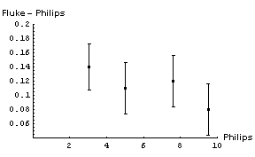
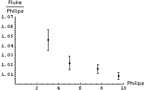
It is not immediately obvious whether the correction factor to be applied to the Philips readings should be an addition of some number or a multiplication by some factor. We will examine both by:

• Subtracting the Fluke reading from the Philips reading.
• Dividing the Fluke reading by the Philips reading.

In both cases we will propagate the errors in quadrature. Here are graphs of the results:

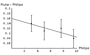
In appears that adding a constant factor to the Philips readings is a reasonable thing to do. The figure to the right shows the Fluke - Philips readings again but with the result of fitting the data to a straight line added. The fit program determined the intercept of the line to be 0.160 ± 0.046 V and the slope to be -0.0075 ± 0.0069.

Thus when we read 6.50 V on the Philips meter we should add a correction factor of :

(0.160 ± 0.046) + (-0.0075 ± 0.0069) × 6.50 = 0.11 ± 0.07V

So the final calibrated result when we read a voltage of 6.50 V on the Philips meter is 6.61 ± 0.07 V. Note that this is much better than the accuracy of the Philips meter, which is ± 0.3 V.

You may wish to know that all of the above numbers are real data, and when the Philips instrument read 6.50 V the Fluke meter measured the same voltage to be 6.63 ± 0.02 V

We conclude this section with some general observations.

First, there are a few companies who have the sales department write their specifications instead of the engineering department. And even reputable companies like Philips and Fluke can not account for the fact that maybe somebody dropped the instrument and broke it.

The calibration discussed above is time consuming, and in the real would only be done if you are going to be using the Philips instrument a lot. If you are only doing one or two measurements and need better accuracy than it supplies, use the better meter instead.

In the calibration, we were combining errors of accuracy using quadrature, although Section 9 clearly states that the rules there are for errors of precision. In Section 11 we justified those rules because we don't know whether a given measurement is higher or lower than the "true" value. That justification means that quadrature was probably the reasonable thing to do in the calibration.

Sometimes we don't care about the accuracy. This is always the case when it is better than the precision of the measurement, but can be true in other cases too. For example, we know that for a current I flowing through a resistor of resistance R, the voltage V across the resistor is given by Ohm's Law:

V = I R

Imagine that to determine the resistance of particular resistor you take data of the voltage for a number of different currents and plot V versus I. The slope of a straight line through the origin and the data will be the resistance R.

If you were doing all the voltage measurements on the 10 volt scale using the Philips meter, its error of accuracy is 0.3 V. This means that all the readings can read, say, 0.3 volts too high. If all the readings are too high or too low by the same amount, this has no effect on the slope and therefore no effect on your determination of the resistance.

This is essentially the situation for Philips meter we have been discussing, the meter almost always read too low by 0.160 V. Put another way, the slope of the fitted calibration line (-0.0075 ± 0.0069) is almost zero with errors.

Question 12.2. Above we said that in determining the resistance, the line should go through the origin as well as the data points. Why? What does it mean physically if the line does not go through the origin?

Question 12.3. How would you calibrate the rulers and/or meter sticks you used in Exercise 12.1?

13 - Rejection of Measurements

Often when repeating measurements, one value appears to be spurious and we would like to throw it out. Also, when taking a series of measurements, sometimes one value appears "out of line". Here we discuss some guidelines on rejection of measurements.

It is important to emphasize that the whole topic of rejection of measurements is awkward. Some scientists feel that the rejection of data is never justified unless there is external evidence that the data in question is incorrect. Other scientists attempt to deal with this topic by using quasi-objective rules such as Chauvenet's Criterion. Still others, often incorrectly, throw out any data that appear to be incorrect. In this section, some principles and guidelines are presented.

First, we note that it is incorrect to expect each and every measurement to overlap within errors. For example, if the error in a particular quantity is characterized by the standard deviation, we only expect 68% of the measurements from a normally distributed population to be within one standard deviation of the mean. Ninety-five percent of the measurements will be within two standard deviations, 99% within three standard deviations, etc., but we never expect 100% of the measurements to overlap within any finite-sized error for a truly Gaussian distribution.

Of course, for most experiments the assumption of a Gaussian distribution is only an approximation.

If the error in each measurement is taken to be the reading error, again we only expect most, not all, of the measurements to overlap within errors. In this case the meaning of "most", however, is vague and depends on the optimism/conservatism of the experimenter who assigned the error.

Thus, it is always dangerous to throw out a measurement. Maybe we are unlucky enough to make a valid measurement that lies ten standard deviations from the population mean. A valid measurement from the tails of the underlying distribution should not be thrown out. It is even more dangerous to throw out a suspect point indicative of an underlying physical process. Very little science would be known today if the experimenter always threw out measurements that didn't match preconceived expectations!

In general, there are two different types of experimental data taken in a laboratory and the question of rejecting measurements is handled in slightly different ways for each. The two types of data are the following:

1. A series of measurements taken with one or more variables changed for each data point. An example is the calibration of a thermocouple, in which the output voltage is measured when the thermocouple is at a number of different temperatures.
2. Repeated measurements of the same physical quantity, with all variables held as constant as experimentally possible. An example is measuring the time for a pendulum to undergo 20 oscillations and repeating the measurement five times, as in Question 10.1.

For a series of measurements (case 1), when one of the data points is out of line the natural tendency is to throw it out. But, as already mentioned, this means you are assuming the result you are attempting to measure. As a rule of thumb, unless there is a physical explanation of why the suspect value is spurious and it is no more than three standard deviations away from the expected value, it should probably be kept. Thus, throwing out a measurement is usually justified only if both of the following are true:

• A definite physical explanation of why the suspect value is spurious is found.
• The suspect value is more than three error bars away from the expected (interpolation/extrapolated) value, and no other measurement appears spurious.

For this case of a series of measurements, there is a whole range of robust fitting techniques which attempt to objectively determine to what degree a single datum may be ignored.

For repeated measurements (case 2), the situation is a little different. Say you are measuring the time for a pendulum to undergo 20 oscillations and you repeat the measurement five times. Assume that four of these trials are within 0.1 seconds of each other, but the fifth trial differs from these by 1.4 seconds (i.e., more than three standard deviations away from the mean of the "good" values). There is no known reason why that one measurement differs from all the others. Nonetheless, you may be justified in throwing it out. Say that, unknown to you, just as that measurement was being taken, a gravity wave swept through your region of space time. However, if you are trying to measure the period of the pendulum when there are no gravity waves affecting the measurement, then throwing out that one result is reasonable. (Although trying to repeat the measurement to find the existence of gravity waves will certainly be more fun!) So whatever the reason for a suspect value, the rule of thumb is that it may be thrown out provided that fact is well documented and that the measurement is repeated a number of times more to convince the experimenter that he/she is not throwing out an important piece of data indicating a new physical process.

14 - Graphical Analysis

So far we have been using arithmetic and statistical procedures for most of our analysis of errors. In this section we discuss a way to use graphs for this analysis.

First, we introduce the use of "error bars" for the graphical display of a data point including its errors. We illustrate for a datapoint where (x, y) = (0.6 ± 0.1, 0.5 ± 0.2). The value of the datapoint, (0.6, 0.5), is shown by the dot, and the lines show the values of the errors. The lines are called error bars.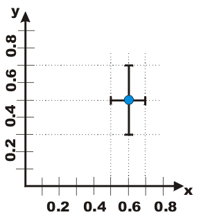

To the right we show data used in the analysis of a Boyle's Law experiment in the introductory Physics laboratory at the University of Toronto. Note the error bars on the graph. Instead of using a computer to fit the data, we may simply take a straight edge and a sharp pencil and simply draw the line that best goes through data points, as shown. Note we have used a red pencil. Recall that the slope is defined as the change in the dependent variable, pV in this case, divided by the change in the independent variable, 1/V in this case. The intercept is defined as the value of the dependent variable when the independent variable is equal to zero. In the graph to the right, the point where the independent variable is equal to zero is not shown. From the drawn line we can calculate that the intercept is 334 and the slope is -49.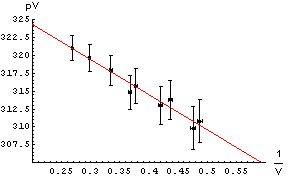

The errors in the determination of the intercept and slope can be found by seeing how much we can "wiggle" the straight edge and still go through most of the error bars. To the right we draw those lines with a blue pencil. The intercepts and slopes of the blue lines, then, allows us to estimate the error in the intercept and slope of the red best match to the data. For this example, this procedure gives an estimate of the error in the intercept equal to ± 4 and the error in the slope equal to ± 10. So finally: .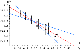

intercept = 334 ± 4
slope = -49 ± 10

Question 14.1. Above we said the blue lines need only go through "most of the error bars." Assuming that the error bars represent standard errors such as the standard deviation, what is the numerical definition of "most"?

Question 14.2. In the first graph above we can not read the intercept directly off the graph because of the scale we have chosen. In the example to the right we can: it is just the point where the line intercepts the pV axis. Why is this graph not as good as the first one?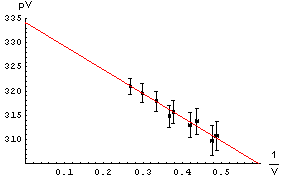

References

Peter L. Bernstein, Against the Gods: The Remarkable Study of Risk (Wiley, 1996 (hardcover), 1998 (paper)), ISBN: 0471121045 (hardcover), ISBN: 0471295639 (paper). The author is an economic consultant who in this book explores the history of the science of statistics. This book was a major motivation for this series of documents and exercises.

John R. Taylor, An Introduction to Error Analysis : The Study of Uncertainties in Physical Measurements, 2nd ed. (Univ. Science Books, 1997), ISBN: 0935702423 (hardcover), ISBN: 093570275X (paper). A classic textbook, used in some introductory Biology labs as well as many labs in Physics and Engineering.

Summary of Formulae

Gaussians

Propagation of Errors of Precision

If or	Then:
If or	Then:
If	Then:
If	Then: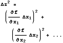

Standard Error of the Mean