Fourier Transform, A Brief Introduction

A “Brief” Introduction to the Fourier Transform

This document is an introduction to the Fourier transform. The level is intended for Physics undergraduates in their 2^nd or 3^rd year of studies. We begin by discussing Fourier series.

We then generalize that discussion to consider the Fourier transform. We next apply the Fourier transform to a time series, and finally discuss the Fourier transform of time series using the Python programming language.

Fourier Series

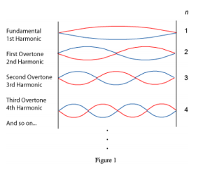We begin by thinking about a string that is fixed at both ends. When a sinusoidal wave is reflected from the ends, for some frequencies the superposition of the two waves will form a standing wave with a node at each end. We characterize which standing wave is set up on the string by an integer n = 1, 2, 3, 4, ... In general n can be any positive integer, so there are in principle an infinite number of possible standing waves. Figure 1 shows the first four possible standing waves.

For a particular standing wave, any point on the string is executing simple harmonic motion, but the amplitude depends on the position on the string. We can write the string’s displacement as a function of position and time, D(x, t), as the product of the amplitude and the harmonic oscillation. For the n-th standing wave:

\[D_n(x ,t ) =A_n (x )cos(\omega_n+\phi_n ) \tag{1}\]

If the length of the string is L, then the amplitude to the n-th standing wave is:

\[A_n(x)=a_{max}sin(2\pi \frac{x}{\lambda_n}) \tag{2}\]

where n is the wavelength of the standing wave, which is:

\[\lambda_n=\frac{2L}{n} \tag{3}\]

So, for n = 1 the wavelength as twice the length of the string. For n = 2 the wavelength equals the length of the string, and so on. This can be easily seen in Figure 1. For a real string, such as on a guitar or violin, the amplitude A_general(x, t) will in general be pretty complicated. However, as Fourier realized long ago, that complicated vibration is just the sum of the possible standing waves. In terms of the amplitude:

\[A_{general}(x)= \sum_{n=1}^{\infty}b_nsin(2\pi \frac{x}{\lambda_n}) \tag{4}\]

The boundary condition that the string is fixed on both ends means that the amplitude varies as a sine function. If the string were not fixed at the ends, the boundary condition would be that at the ends of the strings the vibration will be an anti-node. In this case, the amplitude varies as a cosine function. So a more general form of Equation 4 for any boundary condition is:

\[A_{general}(x)= \sum_{n=1}^{\infty}a_ncos(2\pi \frac{x}{\lambda_n})+ \sum_{n=1}^{\infty}b_nsin(2\pi \frac{x}{\lambda_n}) \]

There is one more subtlety. We have assumed that the oscillations are around y = 0. A more general form would allow for oscillations about some non-zero value. Then we have:

\[A_{general}(x)=\frac{a_0}{2} \sum_{n=1}^{\infty}a_ncos(2\pi \frac{x}{\lambda_n})+ \sum_{n=1}^{\infty}b_nsin(2\pi \frac{x}{\lambda_n}) \]

Finally, we know that:

\[e^{-i\theta}=cos(\theta)-isin(\theta) \tag{5} \]

so we can re-write the Fourier series in terms of complex coefficients cn as:

\[A_{general}(x)= \sum_{n=1}^{\infty}c_n e^{-i(2\pi \frac{x}{\lambda_n})} \tag{6}\]

For the n-th standing wave each point on the string is executing simple harmonic motion with angular frequency \(\omega_n\). Since for any wave the frequency \(f\) times the wavelength \(\lambda\) is equal to the speed of propagation of the wave down the string, we can relate the frequency and period T of the oscillation to the wavelength for the n-th standing wave:

\[\lambda_n f_n=v\]

\[f_n=\frac{\omega_n}{2\pi}=\frac{v}{\lambda_n}\]

\[\omega_n=\frac{nv}{2L} \tag{7}\]

\[T_n=\frac{1}{f_n}=\frac{2L}{nv}\]

Each standing wave will generate a sound wave of the same frequency traveling through the air. We can write the amplitude of the sound wave as a function of time, y_n(t) , at some position away from the string as:

\[y_n(t)=a_{max}sin(2\pi \frac{t}{T_n}+\phi)\]

\[=a_{max}sin(\omega_nt+\phi)\]

Of course, in general the sound wave will be some complicated function of the time, but that complicated function is a sum of the sound waves from the individual standing waves on the string. Thus we can de-compose the sound wave as a function of time the same way we did for the amplitude of the standing wave as a function of position.

\[A_{general}(x)=\frac{a_0}{2} \sum_{n=1}^{\infty}a_ncos(\omega_nt)+ \sum_{n=1}^{\infty}b_nsin(\omega_nt) \tag{8}\]

Musicians call the n = 1 term the fundamental: it represents the note that the string is playing. The terms with n > 1 are called the overtones, and the relative amounts and phases of the overtones determines the timbre of the sound, so that a violin and a Les Paul guitar playing the same note sound different. Integrating sine and cosine functions for different values of the frequency shows that the terms in the Fourier series are orthogonal. In terms of the Kronecker delta:

\[\delta_{nm} \equiv \left\{ \begin{array}{rcl} 1 & m=n \\ 0 & m \neq n \end{array}\right. \]

the orthogonality conditions are:

\[ \int_0^{2pi/\omega_1} sin(n\omega_1t )sin(m\omega_1t )dt =\delta_{nm}\frac{\pi}{\omega_1} \]

\[\int_0^{2pi/\omega_1} cos(n\omega_1t )cos(m\omega_1t )dt =\delta_{nm}\frac{\pi}{\omega_1}\tag{9}\]

\[\int_0^{2pi/\omega_1} sin(n\omega_1t )cos( m\omega_1t )dt =0 ~~Any~ m,n\]

You will want to notice that the limits of the integrations in Equations 9 are from 0 to T₁, the period of the n = 1 standing wave.

Given the function y_general(t), we can find the coefficients of the Fourier series in Equation 8 using the orthogonality conditions to get:

\[a_n=\frac{\omega_1}{\pi}\int_0^{2pi/\omega_1}y_{general}(t) cos(n\omega_1dt )dt\]

\[b_n=\frac{\omega_1}{\pi}\int_0^{2pi/\omega_1} y_{general}(t) sin(n\omega_1dt )dt \tag{9}\]

Fourier Transforms

In Equation 10 we found the coefficients of the Fourier expansion by integrating from 0 to T₁. We could just have well considered integrating from -T₁ / 2 to +T₁ / 2 or even from \(-\infty\) to \(+\infty\) . But what about a non-periodic function over an infinite range? Although we won't go through all of the mathematical details, it is not too difficult to show that we can write the equivalent of Equation 10 for this case using the complex notation introduced in Equation 6 to write:

\[Y(\omega) = \int_{-\infty}^{+\infty} y(t)e^{-i\omega t}dt \tag{11}\]

Equation 11 defines the Fourier transform. Physically we have resolved a single pulse or wave packet y(t) into it frequency components. Notice that Y is only a function of the angular frequency, so we have transformed a function of time into a function of angular frequency. We can also define the inverse Fourier transform which takes a function of angular frequency and produces a function of time:

\[y(t) =\frac{1}{2\pi} \int_{-\infty}^{+\infty} Y(\omega)e^{+i\omega t}d\omega \tag{12}\]

If you look in other sources, you may see other conventions for the Fourier transform and the inverse Fourier transform. Some normalize the integral of Equation 11 by multiplying the integral by 1/ \(\sqrt{2\pi}\) and multiplying the integral in Equation 12 by the same factor of 1/ \(\sqrt{2\pi}\) . Still other sources have the Fourier transform involve a positive exponential, with the inverse transform using the negative exponential. We will always use the conventions of Equations 11 and 12 in this document. Our first example will be 10 oscillations of a sine wave with angular frequency \(\omega\) = 2.5 s^-1

\[y(t) = \left\{ \begin{array}{rcl} sin(2.5t) & -4\pi \leq t \leq +4\pi \\ 0 & |t|>4\pi \end{array}\right. \tag{13}\]

The Fourier transform is:

\[Y(\omega) = \int_{-\infty}^{+\infty} y(t)e^{-i\omega t} dt\]

\[ = \int_{-4\pi}^{+4\pi} sin(2.5t)e^{-i\omega t}dt \tag{14}\]

Since y(t) is a sine function , from Equation 5 we expect the Fourier transform Equation 14 to be purely imaginary.

Figure 2(a) shows the function, Equation 13, and Figure 2(b) shows the imaginary part of the result of the Fourier transform, Equation 14.

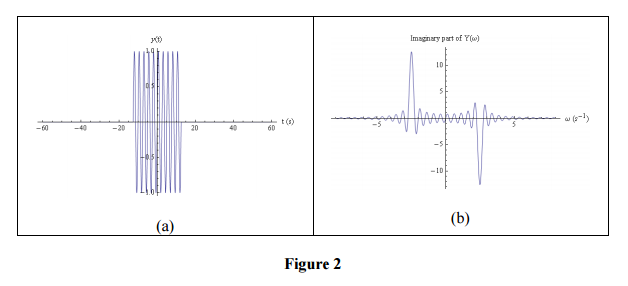
There are at least two things to notice in Figure 2.

First, the Fourier transform has a negative peak at 2.5 s^-1 and a positive peak at –2.5 s^-1. The negative peak at +2.5 s^-1 is minus the sine component of the frequency spectrum. It is negative because we chose the negative exponential for the Fourier transform, Equation 11, and according to Equation 5 the imaginary part is minus the sine component. Signs are always a bit of a pain in Fourier transforms, especially since, as already mentioned, different implementations use different conventions.

The positive peak at –2.5 s^-1 arises because the angular frequency could just as well have a negative value as positive one, but the sine function is anti symmetric, sin(\(\theta\) ) =-sin(\(-\theta\) .

The second thing that you should notice is that there is significant overlap between the curve of the positive angular frequency solution and the negative angular frequency one.

Nonetheless, Figure 2(b) shows that to generate a finite sine wave pulse requires the superposition of a number of frequencies in addition to the frequency of the sine wave itself.

There is also a computational issue of which you should be aware. Although it is possible to evaluate Equation 14 by hand giving a purely imaginary solution, rounding errors mean that doing it with software such as Mathematica will produce small but non-zero real terms. For this case the largest value of the calculated real component of the Fourier transform as evaluated by Mathematica is a negligible -5 x10^-17. This property of software evaluation of Fourier transforms will occur again in this document.

We will now take the Fourier transform of the same sin(2.5t) function, but this time for 30 oscillations.

\[y(t) = \left\{ \begin{array}{rcl} sin(2.5t) & -12\pi \leq t \leq +12\pi \\ 0 & |t|>12\pi \end{array}\right. \tag{15}\]

The Fourier transform is:

\[ = \int_{-12\pi}^{+12\pi} sin(2.5t)e^{-i\omega t}dt \tag{15}\]

Figure 3 shows the function and its Fourier transform.

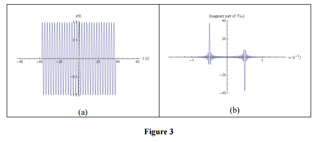
Comparing with Figure 2, you can see that the overall shape of the Fourier transform is the same, with the same peaks at –2.5 s^-1 and +2.5 s^-1, but the distribution is narrower, so the two peaks have less overlap. If we imagine increasing the time for which the sine wave is non-zero to the range \(-\infty\) to \(+\infty\) the width of the peaks will become zero. Physically this means that there is only one frequency component of an infinitely long sine wave pulse, and it is equal to the frequency of the sine wave itself.

In Physics, being able to resolve a signal into its frequency components is immensely useful. However, there is more Physics contained in the Fourier transform.

First, you may have already recognized the shape of the Fourier transforms in Figures 2(b) and 3(b). They are identical to the wave amplitudes of single-slit diffraction. This is not a coincidence. Although we have been thinking of the variable t as time, imagine for a moment that it is a position. Then Equation 13 is describing diffraction through a slit whose width is 8\(\pi\) , while Equation 15 is for a slit whose width is 24\(\pi\) . So the fact that the width of the distribution in Figure 3(b) is narrower than the distribution in Figure 2(b) is telling us that the width of the diffraction pattern for a narrow slit is greater than the width for a wide slit.

Here is some more Physics hidden in the Fourier transform. If we have N oscillations of a sine wave pulse of the form sin(\(\omega\)t) , it is not too difficult to show that the width of the central maximum of the Fourier transform is:

\[\Delta \omega = \frac{\omega_0}{N} \tag{17}\]

If we think about the photon aspect of an electromagnetic sine wave, the energy of the photon is:

\[E_{photon} =hf_0=\hslash \omega_0 \tag{18}\]

But since the frequency of the Fourier transform has angular frequencies in addition to \(\omega_0\) , there is an uncertainty in the true value of the angular frequency. It is fairly reasonable to take value of the uncertainty from the width of the central maximum, Equation 17. So there is an uncertainty in the energy of the photon:

\[E_{photon} =\hslash \Delta \omega \tag{19}\]

\[=\hslash \frac{ \omega_0 }{N}\]

If we are at some position in space, the time t it takes for the wave to pass us is NT₀=N2\(\pi\)/\(\omega_0\) . This is the uncertainty in the time when the photon actually passes us, so:

\[ \Delta t_{photon}=2\pi \frac{N}{\omega_0} \tag{20} \]

The product of these two uncertainties, our uncertainty in the energy of the photon and our uncertainty about when it had that energy, is:

\[ \Delta E_{photon} \Delta t_{photon}= \hslash \frac{ \omega_0 }{N} \times 2\pi \frac{N}{\omega_0} tag{21}\]

Thus the product of the uncertainties is Planck’s constant, independent of the value of the number of oscillations N or the frequency \(\omega_0\) of the sine wave. Heisenberg’s uncertainty principle actually states:

\[ \Delta E_{photon} \Delta t_{photon} \geq \hslash \tag{22}\]

We conclude that the uncertainty principle is related to the Fourier transform.

Time Series

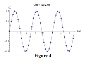Although theorists often deal with continuous functions, real experimental data is almost always a series of discrete data points. For 3 oscillations of the sin(2.5 t) wave we were considering in the previous section, then, actual data might look like the dots in Figure 4. Of course, good data would include errors in at least the dependent variable if not both variables, but we will ignore that in this document. Figure 4 If we have n data points, the data will look like:

\[y_0,y_1,y_2,....,y_{n-1} \tag{23}\]

Such data are called a time series. In a sort-of poor convention, the sampling interval is usually given the symbol \(\Delta\). For the data of Figure 4, \(\Delta\)=0.20 s and n = 38. For any sampling interval, the times corresponding to the data points of Equation 23 are:

\[0,\Delta,2\Delta,....,(n-1)\Delta \tag{24}\]

For time series, we replace the integral in the Fourier transform, Equation 11, with a sum and the differential time dt with the sampling interval \(\Delta\):

\[ Y_j=Y(\omega_j)=(\sum_{k=0}^{n-1}y_k e^{-i\omega_jt_k}) \times \Delta \tag{25} \]

Equation 25 is the discrete Fourier transform. As we shall soon see, we can set the value of \(\Delta\) to 1 without loss of generality.

The inverse discrete Fourier transform gets back the values of y_k with:

\[ y_k= \frac{1}{2\pi}(\sum_{j=0}^{n-1}Y_j e^{+i\omega_jt_k}) \times \delta \omega \tag{26} \]

Soon we will discuss the \(\delta \omega\) factor in Equation 26, which replaces d\(\omega\) in the continuous inverse transform Equation 12.

Counting from 0, as in Equations 23, 24, 25, and 26, may be new to you. In our everyday life we commonly count from 1, as in “one, two, three, …, n”. This is not how counting is done for time series, or many modern computer languages such as C++, Java, and Python, which count as “zero, one, two, … , n – 1”.¹ This can take a bit of time to get used to. This counting issue is why the current year, 2011, is in the 21^st century, not the 20^th.

To actually use Equation 25 or 26, we need to know the times t_k and angular frequencies \(\omega_j\) . The times are just:

\[t_k= k \Delta \tag{27}\]

The determine \(\omega_j\) we will think about Fourier series. The value of \(\omega_0\)= 0 and corresponds to a DC component in the signal. If the signal is periodic with a period \(T=n\Delta\) , then the next value of the angular frequency is:

\[\omega_1=\frac{2\pi}{T}\]

The next term is:

\[\omega_2=2 \times \frac{2\pi}{T}\]

We see, then, that in general:

\[\omega_j=j\frac{2\pi}{T}=j\frac{2\pi}{n\Delta} \tag{28}\]

Using Equation 27 and 28, the discrete Fourier transform Equation 25 becomes:

\[ Y_j=(\sum_{k=0}^{n-1}y_k e^{-i2\pi \frac{jk}{n}}) \times \Delta \tag{29} \]

In the definition of the inverse discrete Fourier transform, Equation 26, the sum is multiplied by \(\delta \omega\), which is how much the angular frequency \(\omega_j\) changes as j goes to j + 1. We have just seen that this is:

\[\delta \omega=\frac{2\pi}{T}=\frac{2\pi}{n\Delta} \tag{30}\]

So the inverse discrete Fourier transform, Equation 26, becomes:

\[ y_k= \frac{1}{n}(\sum_{j=0}^{n-1}Y_j e^{+i2\pi \frac{jk}{n}}) \times \frac{1}{\Delta} \tag{31} \]

Now, when we actually use the discrete Fourier transform, we end up with a series of values \(Y_0,Y_1,Y_2,....,Y_{n-1}\) . If we want to know the frequency of the \(Y_j\) term, we can just use Equation 28. So the factor of \(\Delta\) that multiplies the sum of Equation 29 is not needed, and we just set its value to 1. Similarly, the inverse discrete Fourier transform returns a series of values \(y_0,y_1,y_2,....,y_{n-1}\) and if we want to the know the time of the value of \(y_k\) , we can just use Equation 27. So for the inverse discrete Fourier transform we can similarly just set \(\Delta=1\). So the final form of the discrete Fourier transform is:

\[ Y_j=\sum_{k=0}^{n-1}y_k e^{-i2\pi \frac{jk}{n}} \tag{32} \]

and the inverse discrete Fourier transform is:

\[ y_k= \frac{1}{n}\sum_{j=0}^{n-1}Y_j e^{+i2\pi \frac{jk}{n}} \tag{33} \]

Figure 5 shows the imaginary part of the discrete Fourier transform of the sampled sine wave of Figure 4 as calculated by Mathematica.

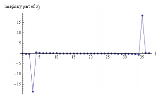
Figure 5. The imaginary part of discrete Fourier transform of 3 cycles of the wave sin(2.5 t) with \(\Delta\)= 0.20 s. The number of samples of the time series n = 38.

There may be a major surprise for you in Figure 5. You can see the negative peak, which for the continuous Fourier transforms Figures 2(b) and 3(b) corresponded to the angular frequency of 2.5 s^-1. But the positive peak, corresponding to the angular frequency of 12 –2.5 s^-1, is now to the far right. What has happened is that the discrete Fourier transform just returns a series of n = 38 values:

\[Y_0,Y_1,Y_3,....,Y_{n-3},Y_{n-2},Y_{n-1} \]

The first 19 of these correspond to the positive angular frequency values of Figures 2(b) and 3(b). The other 19 values, corresponding to the negative angular frequencies, have just been appended to the end of the first 19 values.

Although the discrete Fourier transform shown in Figure 5 was evaluated with Mathematica, this way of handling the negative frequency solutions is standard for most implementations, including Python’s implementation discussed in the next section.2 One reason why is that usually we are not interested in the negative frequency “alias” solution, so can just ignore it or even just throw out the last half of the Fourier transform data.

There may be another small surprise in Figure 5. The amplitude of the sampled sine wave is just 1, but the absolute value of minimum and maximum values of the transform is approximately 19, which is one-half the number of samples n = 38. This is a consequence of the normalization conditions of Equations 32 and 33. A symmetric normalization would multiply the sum by 2/n for the discrete Fourier transform, and replace the 1/n factor for the inverse transform by the same factor of 2/n. Using this convention, the maximum and minimum values would be what you might expect. This was also an issue for the continuous Fourier transforms of the previous section, but we ignored that in the discussion.

The negative peak in the imaginary part of the Fourier transform shown in Figure 5 occurs at the 4^th value, which is j = 3. From Equation 28, this corresponds to an angular frequency of:

\[ \omega_3 =3\frac{2\pi}{n\Delta}=3\frac{2\pi}{3 \times(0.20s)}=2.48s^{-1}\]

It is reasonable to assume that the error in this value of one-half of the change in the value of the angular frequency from j to j +1, \(\delta \omega / 2\) . From Equation 30 this is:

\[ \frac{\delta \omega}{2} =\frac{1}{2}\frac{2\pi}{n\Delta}=3\frac{\pi}{3 \times(0.20s)}=0.41s^{-1}\]

So the frequency corresponding to the peak is:

_{2 Full disclosure: by default Mathematica’s implementation of the discrete Fourier transform does not match the normalization conditions of Equation 32, so I have added a normalization factor to the data of Figure 5 to force it to match the normalization used throughout this document. Python’s implementation, discussed in the next section, does match the conventions of Equations 32 and 33.}

\[\omega_3=(2.48 \pm 0.41)s^{-1} \]

which is well within errors of the actual frequency of the signal, 2.5 s^-1. Increasing the number of samples will reduce the uncertainty in the calculated value of the frequency.

We saw in our discussion of the continuous Fourier transform of a sine function that evaluating the integrals in software gave very small extraneous values for the real parts of the transform. This is also an issue for the discrete Fourier transform, but is compounded by the fact that the signal is sampled and not continuous. For the example of Figure 5, the maximum magnitude of the real part of the Fourier transform is about 8% of the maximum magnitude of the imaginary part. The effect of the sampling time \(\Delta\) on Fourier transforms is an immense topic, which we will not discuss here beyond saying that in general the smaller the sampling time the better.

The actual way that the discrete Fourier transforms, Equations 32 and 32, are implemented means that there is a caveat associated with the statement that the smaller the sampling time the better. If we evaluate Equation 32 using “brute force” we can define:

\[W= e^{-i \frac{2\pi}{n}} \tag{34}\]

Then the discrete Fourier transform becomes:

\[ Y_j=\sum_{k=0}^{n-1}y_k e^{-i2\pi \frac{jk}{n}}=\sum_{k=0}^{n-1}y_k W^{jk} \tag{35} \]

We can think of y_k as a vector of length n, and W as a matrix of dimension \(n \times k\). The multiplication of the two requires n² calculations, and evaluating the sum requires a smaller number of operations to generate the powers of W. Thus the number of calculations necessary to evaluate the Fourier transform is proportional to n². Doubling the number of points in the time series quadruples the time necessary to calculate the transform, and tripling the number of points requires nine times as much time. For large data sets, then, the time necessary to calculate the discrete Fourier transform can become very large.

However, there is a brilliant alternative way of doing the calculation that is was reinvented by Cooley and Tukey in 1965.³ It is called the fast Fourier transform. The idea is that we split the sum into two parts:

_{3 The algorithm was originally invented by Gauss in 1805.}

\[ Y_j=\sum_{k=0}^{n/2-1}y_{2k} e^{-i2\pi \frac{j2k}{n}} + \sum_{k=0}^{n/2-1}y_{2k+1} e^{-i2\pi \frac{j(2k+1)}{n}} \tag{36} \]

The first sum involves the even terms y_2k, and the second one the odd terms y_{(2k + 1)}. Using the definition of W in Equation 34 we can write this as:

\[ Y_j= Y_j^{k~even} +W^k \sum_{k=0}^{n/2-1}y_{2k+1} e^{-i2\pi \frac{jk}{n/2}} \]

\[=Y_j^{k~even} +W^k Y_j^{k~odd} \tag{37}\]

We can apply the same procedure recursively. Eventually, if n is a power of two, we end up with no summations at all, just a product of terms.

An analogy to the algorithm of the fast Fourier transform is a method to determine the number of hairs on your head. Just counting all the hairs would be a very long process. However, imagine that you divide your scalp into two equal pieces. Then the total number of hairs on your head is 2 times the number of hairs in one of the two pieces. If you divide one of those pieces in half, the total number of hairs on your head is 2² times the number in that sample. Dividing that piece in half means that the total is 2³ times the number in the new sample. If you keep dividing the area of your scalp in half a total of M times, then eventually you get down to a small enough piece that you can easily count the number of hairs in it, and the total number of hairs is 2^M times the hairs in the sample area. In the limit where you divide the areas of your scalp enough times that the sample contains just one hair, then the number of hairs on your head is just 2^M .

It turns out that the number of calculations required using the fast Fourier transform is proportional to nlog₂n. So doubling the number of points in the time series only doubles the time necessary to do the calculation, and tripling the number of points increases the time by about 4.75. This is a big win over the brute force method of doing the calculation.

Any competent implementation of the fast Fourier transform does not require that the number of data points in the times series be a power of two, but if not it will need to use some brute force calculations at least at the end. In one test, a time series of e^-t/100 was generated for t from 0 to 1000.001 with \(\Delta\)=0.001. The number of data points was n = 1 000 001, and in one computing environment Mathematica took 0.89 s to calculate the Fourier transform. The value of the last data point is e^1000/100 = 0.0000454, which is nearly zero. 48 575 zeroes were appended to the dataset, so the total length became 1 048 576 = 20 ² . Mathematica took 0.20 s to calculate the Fourier transform of this larger dataset, which is over four times faster. 15

Although speed of calculation is not an issue for the small dataset of 38 samples of a sine wave that we are considering here, the lesson to be learned is that for large datasets for which you wish to use the fast Fourier transform, you should design the experiment so that the number of samples is a power of 2.

Python’s Implementation

The Python programming language has an implementation of the fast Fourier transform in its scipy library. Below we will write a single program, but will introduce it a few lines at a time.

You will almost always want to use the pylab library when doing scientific work in Python, so programs should usually start by importing at least these two libraries:

from pylab import *

from scipy import *

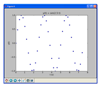
To generate the 38 data points of a time series of sin(2.5 t) with   0.20 as in Figure 4 of the previous section, the following added lines of code will do the trick:

tmin = 0

tmax = 2.4 * pi

delta = 0.2 t = arange(tmin, tmax, delta)

y = sin(2.5 * t)

You can then do a plot of the dataset with:

figure(6)

plot(t, y, 'bo')

title('y(t) = sin(2.5 t)')

xlabel('t (s)')

ylabel('y(t)')

show()

The result is Figure 6 below, which looks similar to Figure 4 of the previous section.

To compute the discrete Fourier transform using the fast Fourier transform routine just requires one line calling the fast Fourier routine fft() from scipy:

Y = fft(y)

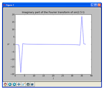
To plot the imaginary parts of the transform, as in Figure 5 of the previous section:

figure(7)

plot(imag(Y))

title(‘Imaginary part of the Fourier transform of sin(2.5 t)’)

xlabel(‘j’)

ylabel(‘Yj’)

show()

As part of the Fourier transform package, scipy includes an implementation of Equation 28 which calculates the frequencies of the transform. It is called fftfreq(), and takes the length of the times series and the sampling interval as its arguments. You should be aware that although the Python routines for the trig functions such as sin() take radians as their arguments, fftfreq() returns frequencies in Hz, not the angular frequencies in s-1. Since everything in this document so far has used angular frequencies, the following lines calculate those angular frequencies:

n = len(y)

# Calculate frequencies in Hz

freq = fftfreq(n, delta)

# Convert to angular frequencies

w = 2 * pi * freq

Notice in the above that we have calculated the number of points in the time series n from the actual time series instead of hard-coding the number, and have similarly used the definition of the time step \(\Delta\)= delta whose value was defined earlier in the code. Both of these are good coding practice.

If we plot Yj versus w, Python and the implementation of fftfreq() are pretty smart, and sorts out the positive and negative angular frequency components automatically.

figure(8)

plot(w, imag(Y))

title('Imaginary part of the Fourier transform of sin(2.5 t)')

xlabel('w (rad/s)')

ylabel('Yj')

show()

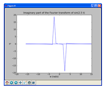
You clearly see the negative peak at \(\omega\)=+2.5 s^-1 and the positive one at \(\omega\)=–2.5 s^-1. You may wish to compare this figure to Figures 2(b) and 3(b) for the continuous Fourier transform.