
8.2: Modeling the Universe (Project)


- Last updated
- Feb 5, 2021
- Save as PDF

( \newcommand{\kernel}{\mathrm{null}\,}\)
Cosmology is the scientific study, and the associated mathematical models, of the universe as a whole. Amazingly, using only a few basic scientific principles one can construct a quantitative model of the universe that agrees surprisingly well with observational data. This model not only is in agreement with current observations, but makes clear predictions for the age of the universe and its future fate.
I. Energy Conservation and the First Friedmann Equation
Consider a large region of our universe, extending a few hundred million light years in all directions from earth. Observationally, portions of the universe this large (or larger) appear isotropic (the same in all directions) and homogeneous (the same from all locations within the region). This implies that if we were to be magically transported to a random location within this region, the universe, on large scales, would look much the same as it does from earth. This observation is consistent with the simplest predictions of relativity, which imply the lack of a “preferred” reference system in the universe. Thus, we can analyze a chunk of the universe centered on the earth (which we can easily observe) and draw conclusions that hold for the entire universe, even the portions beyond our direct observation.
Consider the large region of the universe in Figure 8.2.1, and the one particular galaxy located a distance R from the Milky Way.
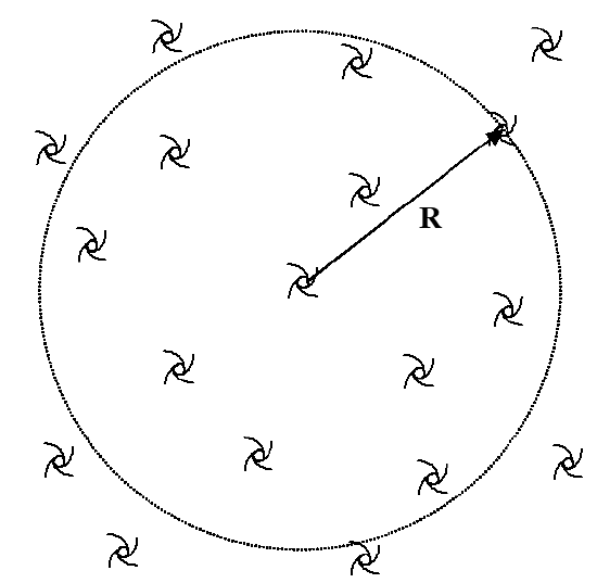
Figure 8.2.1
The total energy of this galaxy is the sum of its kinetic energy and gravitational potential energy.
E=12mv2−GMmR
where, by Gauss’ Law, M is simply the total mass of all of the galaxies within the gaussian sphere of radius R. (The mass of the galaxies outside of the sphere do not contribute to the galaxy’s potential energy.)
In addition to isotropy and homogeneity, another set of observations plays a central role in our understanding of the universe. In 1929, while measuring the velocities of distant galaxies, Edwin Hubble was stunned to find that every galaxy cluster measured was moving directly away from earth. Moreover, he noted that the velocity of each galaxy was directly proportional to its distance from earth, i.e., nearby galaxies are moving away from the earth at relatively low speeds while distant galaxies are moving away very quickly. This is, of course, the first piece of observational evidence in support of the expansion of the universe resulting from the Big Bang.
Mathematically, Hubble’s measurements can be summarized as:
v=dRdt=HR
where H is the Hubble Constant. (The Hubble constant is not actually constant, but rather is a function only of time.)
Putting this together with the energy result yields:
E=12mH2R2−GMnR
Now, what does this equation tell us about the universe? Notice that the energy of this galaxy is the difference between two terms, a positive kinetic energy term related to the Hubble constant and a negative potential energy term related to the total mass between the earth and this galaxy. Since this galaxy, or more properly galaxy cluster, is an isolated system its energy is conserved. Therefore if the total energy is positive today, it will remain positive forever. Thus, as R gets larger and larger (due to Hubble expansion) the potential energy term drops to zero leaving only the positive kinetic energy term. Thus, even as R approaches infinity, the galaxy still has positive kinetic energy. This means that the galaxy will move away from us forever (and the universe will expand forever because there is nothing special about this particular galaxy).
Conversely, if the energy is currently negative, it must always be negative. Since the first term in Equation ??? is proportional to R2, the only way to keep this term from making the entire energy positive is for H to decrease to zero (i.e., the galaxy must stop moving). Once it stops moving, we’ve got problems. The galaxy (and hence the entire universe) will begin to collapse back toward the earth. The situation is exactly analogous to throwing an object upward from the surface of the earth. If the object’s kinetic energy exceeds its gravitational potential energy it will move away forever, if it doesn’t it will come falling back down. To determine the ultimate fate of the universe we need only to determine the value of the Hubble constant (which is relatively easy) and the total mass of our region of the universe (which is where the problems lie …).
Let’s continue to manipulate this equation into the form typically used by cosmologists. The total mass between the earth and the galaxy in question can be written in terms of the mass density within the sphere (ρ) as:
M=ρ(43πR3)
Thus,
E=12mH2R2−4πGmρR232Em=H2R2−8πGρR23
Since E and m (and the number 2) are constants, it would be reasonable to lump them all together into a single constant. Let’s be unreasonable and define them to be the product of two different constants, k and C2, and throw in a negative sign for good measure:
−kC2=2Em
The constant k is the curvature of the universe, and C2 is chosen such that k is equal to either 1, 0, or -1.
- If k=1, the curvature of the universe is positive and space has a spherical shape. This requires E to be negative, and therefore the universe will collapse.
- If k=−1, the curvature of the universe is negative and space has a hyperbolic shape. This requires E to be positive, and therefore the universe will continually expand.
- If k=0, the universe has a flat, Euclidean shape. This requires the universe to have no net energy, and the expansion of the universe asymptotically approaches zero velocity as R approaches ∞.
With this definition, Equation 8.2.6 becomes
−kC2=H2R2−8πGρR23
H2R2=83πGρR2−kC2
(dRdt)2=83πGρR2−kC2
Equation ??? is known as the first Friedmann equation, or the velocity equation, since it is a differential equation for the “velocity” of the expansion of the universe. Although we have used classical physics to derive this result, the result is relativistically correct as long as we interpret ρ as the energy density rather than the mass density of the universe. Also, R is typically referred to as the scale factor of the universe since it applies to any distance measure in the universe, not only the distance between the earth and a particular galaxy. Finally, the constant C can be shown to be everybody’s favorite constant in relativity, the speed of light (c)! Therefore, the first Friedmann equation is:
(dRdt)2=83πGρR2−kc2
II. Work-Energy and the Second Friedmann Equation
In general, the only way a sample of material can change its total energy is by doing work. In general, the change in energy of a system is equal to the negative of its work done (i.e., if it does (positive) work, its change in energy is negative):
ΔE=−work=−∫F(dx)
The force that a system exerts on its surroundings can be represented as the product of its pressure and its area of contact
ΔE=−∫pA(dx)
and the product of the area of contact and the displacement of this area (dx) is the change in volume of the system
ΔE=−∫p(dV)
dE=−pdV
dEdt=−pdVdt
Let’s now examine not a single galaxy a distance R from earth but rather the total energy within the sphere of radius R. With ρ interpreted as the energy density, the total energy within the sphere is simply
E=ρ(43πR3)
Thus,
dEdt=−pdVdtddt(ρ43πR3)=−pddt(43πR3)(dρdt)43πR3+43πρ(3R2dRdt)=−p43π(3R2dRdt)(dρdt)R+ρ(3dRdt)=−p(3dRdt)R(dρdt)=−3(ρ+p)(dRdt)
Let’s call Equation 8.2.25 the cosmological work-energy relation. Great, it has a name, but what does it mean?
Since the universe is expanding,
dRdt>0
and thus
dρdt<0.
Thus, as the universe expands, the energy density decreases (i.e., is diluted by the expansion). Just as the temperature of an ideal gas decreases as it expands, the “temperature” of the universe decreases as it expands.
There is one small twist, however. This story assumes that the energy density and pressure of the universe are positive. If, for example, the pressure is negative (whatever that means) and larger in magnitude than the energy density, you could get the strange result of a universe that expands and increases its energy density. More about this twist later .
So now that we have this lovely equation what should we do with it? How about if we start with a time derivative of the Friedmann Equation (Equation ???):
ddt(dRdt)2=ddt[83πGρR2−kc2]2dRdtd2Rdt2=83πGR2dρdt+83πGρ(2RdRdt)+0
Notice that in the middle term of Equation 8.2.30 is a factor of
Rdρdr.
We can substitute our result from Equation 8.2.25 in for this factor in Equation 8.2.30:
2dRdtd2Rdt2=83πGR[−3(ρ+p)(dRdt)]+83πGρ(2RdRdt)2d2Rdt2=83πGR(−3ρ−3p)+83πGR(2ρ)=83πGR(−ρ−3p)d2Rdt2=−43πGR(ρ+3p)
Equation 8.2.36 is known as the second Friedmann equation, or the acceleration equation, since it is a differential equation for the “acceleration” of the expansion of the universe. It seems to imply that the acceleration of the universe is negative, meaning that the expansion of the universe must slow over time. The sum of the energy density and three times the pressure determines the rate of deceleration, i.e., a universe with lots of energy (and hence mass) has more gravity and slows quicker than a universe with less mass. Two interesting features need attention, however. First, it’s not just matter that creates gravitational attraction since normal positive pressure also slows the expansion of the universe. (This means that a gas in a smaller container will exert more gravitational attraction than the same temperature and mass of gas in a larger container.) Second, if somehow a material had negative pressure, and there was enough of it in the universe, the expansion of the universe could speed up over time.
III. The Equation of State
An equation of state is a relationship between the energy density and pressure of a substance. For example, the ideal gas law,
pV=nRT
is an equation of state because temperature is a measure of energy density. What we are going to do next is find the equation of state for the primary constituents of the universe, photons and matter, and then use the Friedmann equations to calculate what a universe comprised of these two substances would look like.
A. Photons
Imagine a single photon, traveling in the +x-direction with momentum P, striking and elastically rebounding from a surface (Figure 8.2.2). The force exerted on the surface by this photon is given by:
F1photon=ΔPΔt=P−(−P)t=2Pt
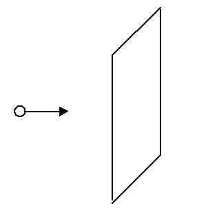
Figure 8.2.2
The total force exerted on the surface by all of the photons in the sample would be the product of the above force and the total number of photons headed in the +x-direction that hit the wall at about the same time. Any photon located within a box of width ct and area A traveling in the +x-direction will hit the wall during this interval (Figure 8.2.3).
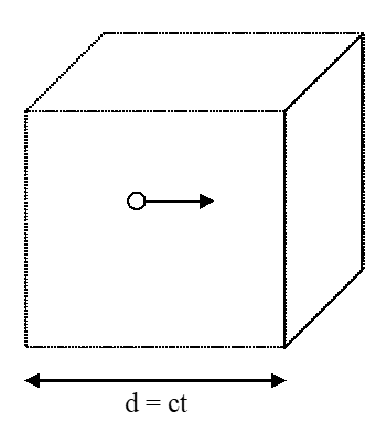
Figure 8.2.3
The total number of photons (N) in the box is that product of the number density of photons (n) and the volume of the box:
N=n(ctA)
We can assume that about ⅓ of these photons are moving in the x-direction (with ⅓ in y and z) and about ½ of the x-photons are moving in the +x-direction (with ½ in –x). Thus:
\begin{align} F _{all\, photons} &= \left( \dfrac{1}{3} \dfrac{1}{2} nctA \right) \left( \dfrac{2P}{t} \right) \\[5pt] &= \left( \dfrac{1}{3} ncAP \right) \end{align}
Thus, the pressure on the surface is:
\begin{align} p &=\dfrac{F}{A} \\[5pt] &= \dfrac{1}{3} nPc \end{align}
Since the energy of a photon is given by
E = Pc
p = \dfrac{1}{3} nE
and energy density is the product of number density and the photon energy,
\rho = nE
we have the equation of state for photons
p_{\gamma} = \dfrac{1}{3} \rho_{\gamma}
B. Matter
The derivation for matter is exactly the same as the derivation for photons, except the “box” has width vt rather than ct. Thus, we are lead to this result:
p_M = \dfrac{1}{3} nPv
Notice that Pv is equal to twice the classical kinetic energy. Under normal conditions, the vast majority of the matter in the universe is moving at non-relativistic speeds. Therefore, the kinetic energy of matter is totally insignificant compared to its rest-mass energy. Thus, the pressure of matter is effectively zero compared to its energy density. This corresponds to an equation of state of
p_M=0
IV. Modeling a Universe of Light and Matter (and the need for more)
A. A Universe of Photons
Consider a universe consisting only of photons. First, apply the cosmological work-energy relation (Equation \ref{work-energy}):
\begin{align} R \left( \dfrac{d\rho}{dt} \right ) &= -3 (\rho-p) \left(\dfrac{dR}{dt} \right) \\[5pt] &= -3 \left(\rho + \dfrac{1}{3} \rho \right) \left( \dfrac{dR}{dt} \right) \\[5pt] &= -3 \left( \dfrac{4}{3} \rho \right) \left( \dfrac{dR}{dt} \right) \\[5pt] &= -4 \rho \left( \dfrac{dR}{dt} \right) \label{eq40} \end{align}
As you can hopefully see, Equation \ref{eq40} is a separable differential equation:
\begin{align} R \left( \dfrac{d\rho}{dt} \right ) &= -4 \rho \left( \dfrac{dR}{dt} \right) \\[5pt] \dfrac{d \rho}{\rho} &= - 4 \dfrac{dR}{dt} \\[5pt] \int \dfrac{d \rho}{\rho} &= \int- 4 \dfrac{dR}{dt} \\[5pt] \ln \rho &= -4 \ln R +C \\[5pt] \rho_\gamma &= \dfrac{C}{R^4} \label{eq45} \end{align}
Equation \ref{eq45} states that as the universe expands (as R increases), the energy density of the photons drops very rapidly. (If you double the radius of the universe, the energy density drops by a factor of 16.) You may have expected that the energy density would drop in inverse proportion to the volume (R^3) (i.e., if you double the radius, you get 8x the volume and 1/8 the energy density). The additional factor diluting the energy density is because the wavelengths of the photons stretch as the universe expands. Since the energy of a photon is inversely proportional to its wavelength, and its wavelength stretches in direct proportion to the scale of the universe, this results in an additional factor of R in the denominator. This “extra” dilution of the energy density of photons as the universe expands has some interesting ramifications we will explore shortly.
Now that we know the relationship between \rho and R, we can solve the Friedmann equation for a universe of photons.
\begin{align} \left( \dfrac{dR}{dt} \right)^2 &= \dfrac{8}{3} \pi G \rho R^2 - kc^2 \\[5pt] &=\dfrac{8}{3} \pi G \left( \dfrac{C}{R^4} \right) R^2 - kc^2 \end{align}
We can ignore the curvature term for two reasons. First, to the limits of our current ability to measure the curvature of the universe, it appears that the universe is flat, so k = 0. Second, even if our measurements are slightly off, when the universe was much smaller than it is now (let R →0), the first term in the Friedmann equation completely dominates the second term. If we are interested in the birth of the universe (when R \approx 0), the curvature of the universe is irrelevant.
Thus,
\begin{align} \left( \dfrac{dR}{dt} \right)^2 &= \dfrac{8}{3} \pi G \left( \dfrac{C}{R^4} \right) R^2 \\[5pt] &= \dfrac{C}{R^2} \label{eq40.5} \end{align}
where I’ve lumped all of the constants together into a “new” constant, but was too lazy to change its symbol. (I’m going to do this a lot so get used to it.)
Taking the square-root of both sides (and being lazy again) of Equation \ref{eq40.5} leaves:
\dfrac{dR}{dt} = \dfrac{C}{R}
This is a separable differential equation:
\begin{align} R\,dR &= C\,dt \\[5pt] \int R\,dR &= \int C\,dt \\[5pt] \dfrac{1}{2} R^2 &= Ct \\[5pt] R &= C\sqrt{t} \end{align}
This says that a universe filled with photons must begin at zero size (R = 0 when t = 0) with a Big Bang-type creation, and then expand as a simple square-root function of time, continuously slowing down in its expansion, but never stopping. (If k really isn’t zero, this would affect the late-time behavior of this universe, but would have no effect on the initial creation and square-root time dependence.)
Now let’s compare this universe to our own. (Of course, there are more than photons in our universe but if this model matches our universe we would say we live in a photon-dominated universe.) To do this, take a time derivative of our model universe:
\dfrac{dR}{dt} = \dfrac{1}{2} Ct^{-1/2}
and pull out a factor of R
\begin{align} \dfrac{dR}{dt} &= \dfrac{1}{2} t^{-1} (Ct^{1/2}) \\[5pt] &= \dfrac{1}{2t} (R) \end{align}
Comparing this to the Hubble law
\dfrac{dR}{dt} = HR
where H is HUbbles constant. This results in
H = \dfrac{1}{2t}
t = \dfrac{1}{2H}
Thus, the Hubble constant is inversely related to the age of the universe. The current value of the Hubble constant is:
H = 70 \dfrac{ km/s}{Mpc} = 2.27 \times 10^{-18} \,s^{-1}
Thus, if our universe is photon-dominated and has this value for the Hubble constant, its age is:
\begin{align} t &= \dfrac{1}{2 (2.27 \times 10^{-18} \,s^{-1}) } \\[5pt] &= 2.2 \times 10^{17} \,s \\[5pt] &\approx 7 \times 10^9 \,yr \end{align}
The current value of the age of the universe is about 13.7 billion years, nearly twice as old as this photon-dominated model. So, we don’t (currently) live in a photon-dominated universe. Obviously, there is a bit of matter around too.
B. A Universe of Matter
Consider a universe consisting only of matter.
Q1
Apply the cosmological work-energy relation to determine the relationship between energy density and scale factor (R).
You should find that the energy density of matter decreases more slowly with expansion than the energy density of photons. This means that in a universe with both matter and photons (such as ours) matter must dominate the universe as R gets larger and larger. Regardless of how much photon energy initially exists, in the limit as R → ∞ this photon energy will disappear, leaving matter to dominate the universe.
Conversely, when the universe was very young (R → 0) the photon energy density increases much faster than the matter energy density. Thus, photons dominate the early universe regardless of the amount of matter in the universe.
In our universe, the transition from a photon-dominated to a matter-dominated universe occurred when the universe was about 70,000 years old. Before this point, the photon densities were so large that no structures (atoms, molecules, etc.) could stably form in the universe and the universe expanded as modeled in the previous section, as t1/2. After this point, the photon energies were diluted by expansion and the universe began its matter-dominated epoch and expanded at a rate you will now calculate.
Q2
Solve the first Friedmann equation to determine the time dependence of the scale factor in a matter-dominated universe.
Q3
Determine the relationship between the age of the universe and the Hubble constant in a matter-dominated universe. Based on the observed Hubble constant, determine the age of our universe if it is matter-dominated.
You should find that for the observed Hubble constant a matter-dominated universe is still only around 9 billion years old. Something is seriously wrong. We know our universe consists of matter and photons, but neither of these two types of model universes can be as old as our universe. Of course, perhaps our measurements of the Hubble constant are incorrect, or perhaps our measurements of the age of the universe are incorrect, or perhaps our measurements of the curvature of space are incorrect, but all of these measurements have been verified by many independent means. So what if none of these sets of measurements are mistaken? One other option is that our universe consists of some other type of substance. (This is not the dark matter astronomers have been looking for for 50 years. This material cannot be matter of any type, luminous or not. It has to be a completely different type of substance.) Amazingly, Einstein predicted the existence of this “substance” nearly a hundred years ago. But before we explore this possibility, let’s look more closely at how the curvature of the universe can affect its age.
C. A Curved Universe of Matter
Let’s revisit the first Friedmann equation (Equation \ref{eq10}) for a matter-dominated universe
\begin{align} \left( \dfrac{dR}{dt} \right)^2 &= \dfrac{8}{3} \pi G \rho R^2 - kc^2 \\[5pt] &= \dfrac{8}{3} \pi G \left( \dfrac{C}{R^3} \right) R^2 - kc^2 \\[5pt] &= \dfrac{C}{R} - kc^2 \end{align}
Ignoring the curvature term hopefully led to a scale factor of the form:
R =\dfrac C t^{2/3}
which is sketched in Figure \PageIndex{4}.
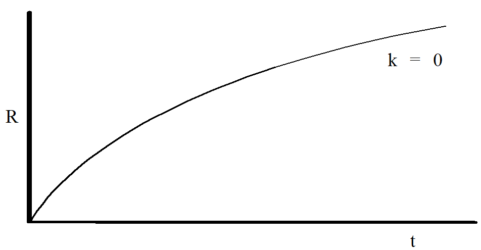
Figure \PageIndex{4}
Q4
What is the expansion velocity for a flat (k = 0) matter-dominated universe as t → ∞?
Now consider a hyperbolic (k = -1) universe. With k = -1, the right-hand side of the Friedmann equation (Equation \ref{eq10}) is now larger than it was for the k = 0 case. Since the left-side of the Friedmann equation is the square of the slope (dR/dt) of the expansion curve, this means that a k = -1 universe is always expanding quicker than a k = 0 universe. Thus, even at t = ∞ a hyperbolic universe is still expanding. Sketch a curve representing a k = -1 universe on the graph above.
What about a spherical (k = +1) universe? With k = +1, the right-hand side of the Friedmann equation is now smaller than it was for the k = 0 case, and thus a k = +1 universe is always expanding slower than a k = 0 universe. Thus, at some time the expansion velocity of a spherical universe must become negative, i.e. the universe must begin to collapse. Sketch a curve representing a k = +1 universe on the graph above.
The graph you’ve constructed above illustrates three different types of universes, all beginning their expansion at the same time. However, what we can directly measure about our universe is not when it began expanding but rather how quickly it is expanding right now. Thus, we know the slope of the expansion curve at the present time.
Matching the slope of the k = 0 universe to its presently measured value resulted in a universe about 9 billion years old. On the graph at below, carefully sketch the curves for k = -1 and k = +1 universes, giving them the correct slope at the present time.
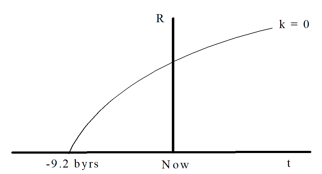
Figure \PageIndex{5}
Q5
Given the current value of the Hubble constant, which type of universe (k = ±1 or 0) is the oldest? Carefully explain your answer.
V. Vacuum Energy
A. Justification
Let’s assume empty space has a non-zero energy density. This is not the energy of something that occupies the space, but rather the energy of the space itself, an inherent property of the space. Why should we make this assumption? The best justification comes from quantum mechanics, where even apparently empty space should not have an energy density of precisely zero. An energy density of exactly zero, with no uncertainty, would seem to be in contradiction with the energy-form of Heisenberg’s uncertainty principle. Quantum mechanics seems to predict that empty space is continually filled with virtual particles whose net energy density is non-zero.
Einstein, working before the advent of quantum mechanics and Hubble’s discovery of an expanding universe, assumed space had a non-zero energy density, which he termed the cosmological constant, for totally different reasons. Because he realized that a universe of only matter and photons would have to be expanding or contracting, and there appeared to be no evidence for universal expansion or contraction, he examined the equations of general relativity and realized that energy of this form could counteract the effects of matter and photons and keep the universe static.
B. Equation of State for Vacuum Energy
The fundamental attribute of vacuum energy density is that it has a constant value, governed by quantum mechanics and independent of whatever else is happening in that region of space. Therefore, if we apply the cosmological work-energy relation (Equation \ref{work-energy}) to vacuum energy:
\begin{align} R \left( \dfrac{d\rho}{dt} \right) &= -3 (\rho + p) \left( \dfrac{dR}{dt} \right) \\[5pt] R(0) &= -3 (\rho + p) \left( \dfrac{dR}{dt} \right) \\[5pt] 0 &= -3 (\rho + p) \left( \dfrac{dR}{dt} \right) \end{align}
Since the universe is expanding
\dfrac{dR}{dt} \neq 0,
so,
\begin{align} 0 &= \rho + p \\[5pt] \rho_V &= -p_V \end{align}
Thus, a positive vacuum energy density results in a negative pressure, and all the crazy results I alluded to earlier in this activity. Also, notice that unlike matter or photon energy densities, vacuum energy density does not decrease as the universe expands. Thus, if there is any non-zero value of vacuum energy in the universe, it will ultimately dominate the universe.
Before we describe how a vacuum-dominated universe behaves, let’s see how Einstein used vacuum energy to “stabilize” the universe.
C. Vacuum Energy and a Static Universe
Examine the second Friedmann equation (Equation \ref{2ndFriedman}) for the acceleration of the universe:
\dfrac{d^R}{dt^2} = -\dfrac{4}{3} \pi GR (\rho+3p)
For a matter-dominated or photon-dominated universe, the universe has a negative acceleration and is either slowing down during its expansion or speeding up during its collapse. Neither of these possibilities seemed possible to Einstein. Therefore, he concocted a universe with both matter and vacuum energy. This leads to a Friedmann equation:
\begin{align} \dfrac{d^2R}{dt^2} &= -\dfrac{4}{3} \pi GR (\rho_M+3(0)) -\dfrac{4}{3} \pi GR (\rho_V + 3(-p_V)) \\[5pt] &= -\dfrac{4}{3} \pi GR ( \rho_M - 2 \rho_V) \end{align}
In this combination universe, the acceleration can be zero if (and only if) the matter energy density is exactly equal to twice the vacuum energy density. This precise balance would seem to lead to the static universe that Einstein (and all of his contemporaries) believed in.
However, this balance is unstable. Although the energy densities could have this perfect proportion averaged over a large volume of the universe, there would almost certainly have to exist small regions in which, for example, the mass density was a tiny bit larger than twice the vacuum density. These regions would then start to collapse, which would further increase the mass density, which would accelerate the collapse, which would further increase the mass density, which … etc. In a region in which the mass density was slightly smaller than twice the vacuum density, the opposite would happen. The positive acceleration in these regions would cause them to expand, which would reduce the mass density, which would accelerate the expansion, etc. A perfectly static universe is impossible, it would immediately be filled with rapidly expanding and contracting sub-regions. Einstein’s goal of a universe stabilized against collapse by the negative pressure of vacuum energy density is impossible.
Q6
Imagine a universe with both photons and vacuum energy. What relationship between photon energy density and vacuum energy density will result in a universal acceleration of zero? Is this universe stable or unstable?
D. The Vacuum-Dominated Universe
7. Solve the first Friedmann equation to determine the time dependence of the scale factor in a vacuum-dominated universe.
The Vacuum-Dominated universe is a seriously strange universe, termed the deSitter universe after the first physicist to clearly describe its properties. Perhaps the strangest aspect of this space is that it was never “created”. At t = 0, the space has finite size, so there is no special Big Bang singularity of creation. Moreover, the space has a finite, positive size regardless of how far back in time you go (let t →-∞). The Hubble constant tells us nothing about this space’s age (as it does for the photon and matter-dominated spaces) because the space has always existed. In fact, the Hubble constant is simply the argument in the exponential expansion of the scale factor,
R = A e^{Ht}
and is not only a spatial constant, but a temporal constant as well. This means that not only does the deSitter universe look the same at every point in space it also looks the same at every point in time (unlike the photon and matter universes which clearly show signs of “aging”).
Of course, we don’t live in a pure deSitter universe, because obviously matter and photons exist in our universe, so how do we take the three models we’ve developed and use them to describe our universe?
E. Our Universe
Our universe consists of photons, matter and (almost assuredly) vacuum energy. Regardless of the exact proportions of these three types of energy, the story of the universe’s expansion neatly divides into three clear stages. In the early universe, photons dominate, even in the presence of vacuum energy, since photon energy density rises without limit as R → 0:
\rho_V = \dfrac{C}{R^4}
while vacuum energy remains constant. Thus, during the early days of our universe (but maybe not the earliest fractions of a second) the universe behaves like a simple photon-only universe, expanding as t^{1/2}. Then, as the photons dilute, matter takes over, slightly altering the expansion rate, but the universe is still slowing in its expansion. Finally, ultimately, vacuum energy takes over. Our universe will begin to accelerate in its expansion, ultimately becoming indistinguishable from the exponentially expanding deSitter universe. The first evidence for this accelerated expansion was collected in the 1990s, and it now appears that several billion years ago our universe began to make its transition to the vacuum-dominated phase.
F. Vacuum Energy and the Creation of the Universe
Within the limits of observational measurements, our universe is flat. This flatness requires a very specific value of energy density, termed the critical density (\rho_C). The value of the critical density can be determined from the first Friedmann equation:
\begin{align} \left( \dfrac{dR}{dt} \right)^2 &= \dfrac{8}{3} \pi G \rho R^2 - kc^2 \\[5pt] \left( \dfrac{dR}{dt} \right)^2 &= \dfrac{8}{3} \pi G \rho_C R^2 - 0 \\ \dfrac{\left( \dfrac{dR}{dt} \right)^2}{R^2} &= \dfrac{8}{3} \pi G \rho_C \\[5pt] H^2 &= \dfrac{8}{3} \pi G \rho_C \\[5pt] \rho_C &= \dfrac{3H^2}{8\pi G} \end{align}
If the energy density of the universe is not equal to this precise value, the universe will not be flat.
\begin{align} \left( \dfrac{dR}{dt} \right)^2 &= \dfrac{8}{3} \pi G \rho R^2 - kc^2 \\[5pt] \dfrac{\left( \dfrac{dR}{dt} \right)^2}{R^2} &= \dfrac{8}{3} \pi G \rho - \dfrac{kc^2}{R} \\[5pt] H^2 - \dfrac{8}{3} \pi G \rho &= - \dfrac{kc^2}{R} \end{align}
Now examine the Friedmann equation again, this time for arbitrary curvature:
H^2 - \dfrac{8}{3} \pi G \rho = \dfrac{kc^2}{R^2}
Now multiply both sides by 3/8 \pi G and use the definition of critical density derived above:
\dfrac{3}{8\pi G} \left( H^2 - \dfrac{8}{3} \pi G \rho \right) = - \dfrac{ 3 kc^2}{8 \pi GR^2}
\rho_C- \rho = - \dfrac{3kc^2}{8 \pi G R^2}
and divide both sides by the energy density:
\begin{align} \dfrac{\rho_C- \rho}{\rho} &= - \dfrac{3kc^2}{8 \pi \rho G R^2} \\[5pt] \dfrac{\rho- \rho_C}{\rho} &= \dfrac{C}{ \rho R^2} \label{Flat} \end{align}
Equation \ref{Flat} relates or the fractional difference between the energy density in our universe and the critical energy density needed for flatness. The important aspect of this equation is that this difference changes as the scale of the universe changes.
If matter or photons dominate the universe near creation, let’s examine how this fractional difference changes. Since matter density scales with the expansion of the universe as:
\rho_M = \dfrac{C}{R^3}\label{eq60}
the right-hand side of Equation \ref{eq60} grows as the universe expands:
\dfrac{ \rho - \rho_C}{\rho} =\dfrac{C}{\left(\dfrac{C}{R^3} \right) R^2} \approx R
Since photon density scales with the expansion of the universe as:
\rho_\gamma = \dfrac{C}{R^4} \label{eq62}
the right-hand side of Equation \ref{eq62} grows as the universe expands:
\dfrac{ \rho - \rho_C}{\rho} =\dfrac{C}{\left(\dfrac{C}{R^4} \right) R^2} \approx R^2
Thus, in a universe dominated by matter and photons, the difference between the density of the universe and the critical density will increase as the universe expands. This is equivalent to saying that the flatness of the universe is unstable, in that the universe becomes less flat as it expands. Thus, if the universe is observationally close to flat today it must have been extremely close to flat at creation. How close? Observationally, the universe is within ±1\% of flatness today. Scaling backwards in time, it must have been within ±10^{-60}\% of flatness near creation! This is an insanely precise value of energy density and, given natural variations in energy density in different regions of the universe, there is no feasible way in which a matter and photon dominated universe as large as ours can be flat. This is termed the Flatness Problem in cosmology and requires some sort of resolution.
I should point out that the vacuum dominated phase we are currently in does not resolve this problem. The curvature of the universe is measured by observing the microwave background radiation, emitted when the universe was about 400,000 years old. Thus, the universe was flat long before the current vacuum dominated phase.
However, the proposed resolution does involve vacuum energy. Imagine very early in the history of the universe (and I mean VERY early, like 10-34 s after “creation”) a vacuum energy density larger than the matter or photon energy densities. (This is not the same vacuum energy density driving the current accelerated expansion of the universe. The current vacuum energy density does not dominate the universe until after matter and photon energies dilute over several billion years.) This vacuum energy density is either a short-term “release” of vacuum energy, analogous to the energy released when a system goes through a phase transformation, or the energy associated with the vacuum being in a higher energy state than it currently is in, analogous to the higher energy states allowed electrons in an atom. Either way, if vacuum energy dominates the very early universe, we can again examine our flatness equation. Since vacuum energy is constant during this time interval:
\rho_V = C
the right-hand side of the flatness equation (Equation \ref{Flat} decreases as the universe expands:
\dfrac{\rho - \rho_C}{\rho} = \dfrac{C}{(C)R^2} \approx \dfrac{1}{R^2}
Thus, vacuum energy makes the universe more flat as it expands! Regardless of the initial curvature of the universe, if it is dominated by vacuum energy near its birth it will emerge almost perfectly flat. This is, as mentioned before, in strong agreement with measurements of our universe. This process, in which a very early burst of accelerated expansion due to vacuum energy flattens our universe is termed inflation. (Inflation also explains a number of other features of our universe that more simple models cannot explain.)
In addition to solving the flatness problem, inflation (and vacuum energy) may also provide the answer to the most fundamental question in cosmology, “How was the universe created?” Remember that a pure, vacuum dominated space has no “time” of creation, it exists eternally. Sometimes termed eternal inflation, this model proposes an eternally inflating vacuum-energy dominated space, in which the vacuum in certain sub-regions occasionally decays into a lower energy state, creating universes such as ours (and probably many not so similar to ours). Obviously, the scope of this model is a bit beyond the level of this course.