
19.10: Examples of Cycloidal Motion in Physics


- Last updated
- Aug 8, 2022
- Save as PDF

( \newcommand{\kernel}{\mathrm{null}\,}\)
Several examples of cycloidal motion in physics come to mind. One is the nutation of a top, which is described in Section 4.10 of Chapter 10. Earth’s axis nutates in a similar fashion. Another well known example is the motion of an electron in crossed electric and magnetic fields. This is described in Chapter 8 of the Electricity and Magnetism section of these notes. In cosmology, if the mean density of the Universe is low, the Universe expands indefinitely, but, if the density is higher than a certain critical density, the (dimensionless) scale factor R of the Universe expands and contracts with time t according to the following parametric cycloidal equations:
R=Ω02(Ω0−1)(1−cos2θ),
t=Ω02(Ω0−1)3/2(2θ−sin2θ).
Here t is expressed in units of the reciprocal of the present Hubble constant, and Ω0 is the ratio of the present density of the Universe to the density required to “close” the Universe.
A less well known example concerns the propagation of sound in the atmosphere. In the troposphere, which is the lower part of the atmosphere up to about 11 km, the temperature decreases roughly linearly with height. In that case sound travels through the troposphere in a cycloidal path. The speed of sound in a gas is proportional to the square root of the temperature. (If you are wondering how it depends on pressure P and density ρ, the answer is that it depends on the ratio P/ρ - and this ratio is proportional to the temperature.) In any case, if the temperature decreases linearly with height, the sound speed v varies with height y as
v=v0√1−cy
where c is a constant, equal to about 0.023 km−1.Now to trace a sound ray through the atmosphere, we have to understand how the direction of propagation changes as the sound passes through layers of air of different temperature. This is governed, as with light, by Snell’s law (see figure XIX.11):
dvv=−tanψdψ
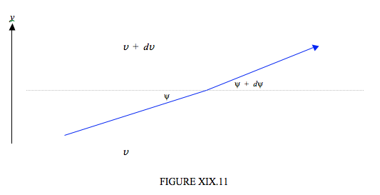
Snell’s law states that when sound (or light) enters a slower medium (i.e. one in which the speed of propagation is slower) it is bent towards the normal. I have drawn figure XIX.11 to represent the situation in the troposphere where the temperature (and hence the sound speed v) decreases with height. That is, dv/dy is negative. In other words dv in figure XIX is negative, and Equation 19.10.4 indicates that dψ is positive, as drawn. In case you do not recognize this differential form of Snell’s law, try integrating it from v1 to v2 and from ψ1 to ψ2, and it should assume its more familiar integral form. If you now eliminate v between Equations 19.10.3 and 19.10.4, you will get a differential relation between y and ψ, which, upon integration, becomes
cy=1−cos2ψcos2ψ0
where ψ0 is the ground-level value of ψ. If we introduce
a=12ccos2ψ0,
equation 19.10.5 can be conveniently re-written
y=2a(sin2ψ−s∈2ψ0)=2a(cos2ψ0−cos2ψ
Now tanψ=dy/dx, and elimination of y between this and Equation 19.10.7 will give a differential relation between x and ψ, which, upon integration, becomes
x=a[2(ψ−ψ0)+sin2ψ−sin2ψ0].
Equations 19.10.7 and 19.10.8 are the parametric equations of the sound path through the troposphere, and describe a cycloid.
If x = 2.0 and y = 1.6, what are ψ and ψ0?
Solution
I make it ψ=69∘,ψ0=15∘52′.