4.10: The Top

We have classified solid bodies technically as symmetric, asymmetric, spherical and linear tops, according to the relative sizes of their principal moments of inertia. In this section, or at least in the title of this section, I mean “top” in the nontechnical sense of the child’s toy – that is to say, a symmetric body, pointed at one end, spinning around its axis of symmetry, with the pointed end on the ground or on a table. Technically, it is a “heavy symmetric top with one point fixed.”

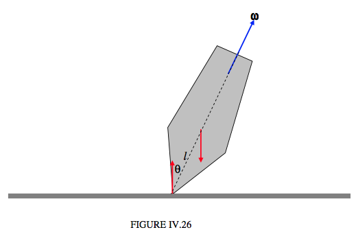
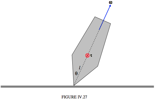
I have drawn it is Figure IV.26, spinning about its symmetry axis, which makes an angle $\theta$ with the vertical. The distance between the centre of mass and the point of contact with the table is l. It has a couple of forces acting on it – its weight and the equal, opposite reaction of the table. In Figure IV.27, I replace these two forces by a torque, $\boldsymbol\tau$, which is of magnitude $Mgl\sin\theta$.

Note that, since there is an external torque acting on the system, the angular momentum vector is not fixed.

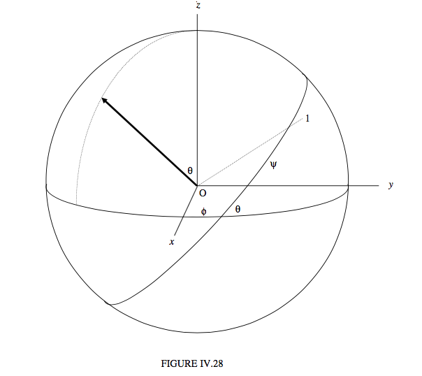
Before getting too involved with numerous Equations, let’s spend a little while describing qualitatively the motion of a top, and also describing the various coordinate systems and angles we shall be discussing. First, we shall be making use of a set of space-fixed coordinates. We’ll let the origin $O$ of the coordinates be at the (fixed) point where the tip of the top touches the table. The axis $Oz$ points vertically up to the zenith. The $Ox$ and $Oy$ axes are in the (horizontal) plane of the table. Their exact orientation is not very important, but let’s suppose that $Ox$ points due south, and $Oy$ points due east. $Oxyz$ then constitutes a right-handed set. We’ll also make use of a set of body-fixed axes, which I’ll just refer to for the moment as 1, 2 and 3. The 3-axis is the symmetry axis of the top. The 1- and 2-axes are perpendicular to this. Their exact positions are not very important, but let’s suppose that the 31-plane passes through a small ink-dot which you have marked on the side of the top, and that the 123 system constitutes a right-handed set.

We are going to describe the orientation of the top at some instant by means of the three Eulerian angles $\theta$, $\phi$ and $\psi$ (see Figure IV.28). The symmetry axis of the top is represented by the heavy arrow, and it is tipped at an angle $\theta$ to the $z$-axis. I’ll refer to a plane normal to the axis of symmetry as the “equator” of the top, and it is inclined at $\theta$ to the $xy$-plane. The ascending node of the equator on the $xy$-plane has an azimuth $\phi$, and $\psi$ is the angular distance of the 1-axis from the node. The azimuth of the symmetry axis of the top is $\phi$ - 90 ° = $\phi$ + 270°.

Now let me anticipate a bit and describe the motion of the top while it is spinning and subject to the torque described above.

The symmetry axis of the top is going to precess around the $z$-axis, at a rate that will be described as $\dot{\phi}$. Except under some conditions (which I shall eventually describe) this precessional motion is secular. That means that $\phi$ increases all the time – it does not oscillate to and fro. However, the symmetry axis does not remain at a constant angle with the $z$-axis. It oscillates, or nods, up and down between two limits. This motion is called nutation (Latin: nutare, to nod). One of our aims will be to try to find the rate of nutation $\dot{\phi}$ and to find the period and amplitude of the nutation.

It may look as though the top is spinning about its axis of symmetry, but this isn’t quite so. If the angular velocity vector were exactly along the axis of symmetry, it would stay there, and there would be no precession or nutation, and this cannot be while there is a torque acting on the top. An exception would be if the top were spinning vertically ($\theta$ = 0), when there would be no torque acting on it. The top can in fact do that, except that, unless the top is spinning quite fast, this situation is unstable, and the top will tip away from its vertical position at the slightest perturbation. At high spin speeds, however, such motion is stable, and indeed one of our aims must be to determine the least angular speed about the symmetry axis such motion is stable.

However, as mentioned, unless the top is spinning vertically, the vector $\omega$ is not directed along the symmetry axis. We’ll call the three components of $\omega$ along the three body- fixed axes $\omega_{1}$, $\omega_{2}$ and $\omega_{3}$, the last of these being the component of $\omega$ along the symmetry axis. One of the things we shall discover when we proceed with the analysis is that $\omega_{3}$ remains constant throughout the motion. Also, you should be able to distinguish between $\omega_{3}$ and $\dot{\psi}$. These are not the same, because of the motion of the node. In fact you will probably understand that $\psi = \omega_{3} - \dot{\phi} \cos \theta$. Indeed, we have already derived the relations between the component of the angular velocity vector and the rate of change of the Eulerian angles – see Equations 4.2.1 ,2 and 3. We shall be making use of these relations in what follows.

To analyse the motion of the top, I am going to make use of Lagrange’s Equations of motion for a conservative system. If you are familiar with Lagrange’s Equations, this will be straightforward. If you are not, you might prefer to skip this section until you have become more familiar with Lagrangian mechanics in Chapter 13. However, I introduced Lagrange’s Equation briefly in Section 4.4, in which Lagrange’s Equation of motion was given as

$$\ \frac{d}{dt} \left(\frac{\partial T}{\partial \dot{q}_{j}}\right) - \left(\frac{\partial T}{\partial \dot{q}_{j}}\right) = P_{j}. \tag{4.10.1}\label{eq:4.10.1}$$

Here $T$ is the kinetic energy of the system. $P_j$ is the generalized force associated with the generalized coordinate $q_j$. If the force is a conservative force, then $P_j$ can be expressed as the negative of the derivative of a potential energy function:

$$\ P_{j} = - \left(\frac{\partial V}{\partial q_{j}}\right) \tag{4.10.2}\label{eq:4.10.2}$$

Thus we have Lagrange’s Equation of motion for a system of conservative forces

$$\ \frac{d}{dt}\left(\frac{\partial V}{\partial \dot{q_{j}}}\right) - \frac{\partial V}{\partial q_{j}} = - \frac{\partial V}{\partial q_{j}} \tag{4.10.3}\label{eq:4.10.3}$$

Thus, in solving problem in Lagrangian dynamics, the first line in our calculation is to write down an expression for the kinetic energy. The first line begins: “$T = ...$”.

In the present problem, the kinetic energy is

$$\ T = \frac{1}{2} I_{1}(\omega^{2}_{1} + \omega^{2}_{2}) + \frac{1}{2} I_{3}\omega^{2}_{3} \tag{4.10.4}\label{eq:4.10.4}$$

Here the subscripts refer to the principal axes, 3 being the symmetry axis. The Eulerian angles $\theta$ and $\phi$ are zenith distance and azimuth respectively of the symmetry axis with respect to laboratory fixed (space fixed) axes. The Eulerian angle $\psi$ is measured around the symmetry axis. The components of the angular velocity are related to the rates of change of the Eulerian angles by previously derived formulas (Equations 4.2.1,2,3), so the $\dot{\theta} , \dot{\phi}$ and $\dot{\psi }$.

$$\ T = \frac{1}{2} I_{1}(\dot{\theta}^{2} + \dot{\phi}^{2} \sin^{2} \theta) + \frac {1}{2} I_{3} (\dot{\psi} + \dot{\phi} \cos \theta)^{2} \tag{4.10.5}\label{eq:4.10.5}$$

The potential energy is

$$\ V = Mgl\cos\theta + constant. \tag{4.10.6}\label{eq:4.10.6}$$

Having written down the expressions for the kinetic and potential energies in terms of the Eulerian angles, we are now in a position to apply the Lagrangian Equations of motion 4.10.3 for each of the three coordinates. We’ll start with the coordinate $\phi$. The Lagrangian Equation is

$$\ \frac{d}{dt}(\frac{\partial T}{\partial \dot{\phi}}) - \frac{\partial T}{\partial \phi} = -\frac{\partial V}{\partial \phi} \tag{4.10.7}\label{eq:4.10.7}$$

We see that $\frac{\partial T}{\partial \phi}$ and $\frac{\partial V}{\partial \phi}$ are each zero, so that $\frac{d}{dt}\frac{\partial T}{\partial \phi} = 0,$ or $\frac{\partial T}{\partial \phi}$ = constant. This has the dimensions of angular momentum, so I’ll call the constant L₁. On evaluating the derivative $\frac{\partial T}{\partial \phi}$, we obtain for the Lagrangian Equation in $\phi$:

$$\ I_{1} \dot{\phi}sin^{2}\theta + I_{3} \dot{\phi}\cos^{2}\theta+ I_{3} \dot{\psi}\cos\theta = L_{1} \tag{4.10.8}\label{eq:4.10.8}$$

I’ll leave the reader to carry out exactly the same procedure with the coordinate $\psi$. You’ll quickly conclude that $\frac{\partial T}{\partial \psi}$= constant, which has the dimensions of angular momentum, so call it $L_{3}$, and you will then arrive at the following for the Lagrangian Equation in $\psi$:

$$\ I_{3}(\psi + \dot{\phi} \cos \theta) = L_{3} \tag{4.10.9}\label{eq:4.10.9}$$

But the expression in parentheses is equal to $\omega_{3}$ (see Equation 4.2.3, although we have already used it in Equation $\ref{eq:4.10.5}$), so we obtain the result that $\omega_{3}$, the component of the angular velocity about the symmetry axis, is constant during the motion of the top. It would probably be worth the reader’s time at this point to distinguish again carefully in his or her mind the difference between $\omega_{3}$ and $\dot{\psi}$.

Eliminate $\dot{\psi}$ from Equations $\ref{eq:4.10.8}$ and $\ref{eq:4.10.9}$:

$$\ \dot{\phi} = \frac{L_{1} - L_{3} cos \theta} {I_{1}\sin^{2}\theta} \tag{4.10.10}\label{eq:4.10.10}$$

This Equation tells us how the rate of precession varies with $\theta$ as the top nods or nutates up and down.

We could also eliminate $\dot{\phi}$ from Equations $\ref{eq:4.10.8}$ and $\ref{eq:4.10.9}$:

$$\ \dot{\psi} = \frac{L_{3}}{I_{3}} - \frac{(L_{1}-L_{3} \cos\theta)\cos\theta}{I_{1}\sin^{2}\theta} \tag{4.10.11}\label{eq:4.10.11}$$

The Lagrangian Equation in $\theta$ is a little more complicated, but we can obtain a third Equation of motion from the constancy of the total energy:

$$\ \frac{1}{2} I_{1} (\dot{\theta}^{2} + \dot{\phi}^{2}\sin^{2}\theta) + \frac{1}{2} I_{3}(\dot{\psi}+\dot{\phi}\cos\theta)^{2}+Mgl\cos\theta = E. \tag{4.10.12}\label{eq:4.10.12}$$

We can eliminate $\dot{\phi}$ and $\dot{\psi}$ from this, using Equations $\ref{eq:4.10.10}$ and $\ref{eq:4.10.11}$, to obtain an Equation in $\theta$ and the time only. After a little algebra, we obtain

$$\ \dot{\theta}^{2} = A - B\cos\theta - \left(\frac{L_{1}-L_{3} \cos\theta}{I_{1} \sin\theta}\right)^{2}, \tag{4.10.13}\label{eq:4.10.13}$$

where

$$\ A = \frac{1}{I_{1}}\left(2E - \frac{L^{2}_{3}}{I_{3}}\right) \tag{4.10.14}\label{eq:4.10.14}$$

and

$$\ B = \frac{2Mgl}{I_{1}} \tag{4.10.15}\label{eq:4.10.15}$$

The turning points in the $\theta$-motion (i.e. the nutation) occur where $\dot{\theta} = 0$. This results (after some algebra! – but quite straightforward all the same) in a cubic Equation in $c = \cos\theta$:

$$\ a_{0} = a_{1}c + a_{2}c^{2} + Bc^{3} = 0 \tag{4.10.16}\label{eq:4.10.16}$$

where

$$\ a_{0} = A - \left(\frac{L_{1}}{I_{1}}\right)^{2} = \frac{2E}{I_{1}} - \frac{L_{3}^{2}}{I_{1}I_{3}}- \frac{L_{1}^{2}}{I_{1}^{2}}, \tag{4.10.17}\label{eq:4.10.17}$$

$$\ a_{1} = \frac{2L_{1}L_{3}}{I^{2}_{1}} - B = \frac{2L_{1}L_{3}}{I^{2}_{1}} - \frac{2Mgl}{I_{1}} \tag{4.10.18}\label{eq:4.10.18}$$

and

$$\ a_{2} = -A - \left(\frac{L_{3}}{I_{1}}\right)^{2} = -\left[\frac{2E}{I_{1}} - \frac{L^{2}_{3}}{I_{1}I_{3}}- \left(\frac{L_{3}}{I_{1}}\right)^{2}\right] \tag{4.10.19}\label{eq:4.10.19}$$

Now Equation $\ref{eq:4.10.16}$ is a cubic Equation in $\cos \theta$ and it has either one real root or three real roots, and in the latter case two of them or all three might be equal. We must also bear in mind that $\theta$ is real only if $\cos \theta$ is in the range −1 to+1. We are trying to find the nutation limits, so we are hoping that we will find two and only two real values of $\theta$. (If the tip of the top were poised on top of a point – e.g. if it were poised on top of the Eiffel Tower, rather than on a horizontal table − you could have $\theta$ > 90°.)

To try and understand this better, I constructed in my mind a top somewhat similar in shape to the one depicted in Figures IV.25 and 26, about 4 cm diameter, 7 cm high, made of brass. For the particular shape and dimensions that I imagined, it worked out to have the following parameters, rounded off to two significant Figures:

M=0.53 kg l= 0.044 m I₁ = 1.7×10⁻⁴ kg m² I₃ = 9.8×10⁻⁵ kg m²

I thought I’d spin the top so that $\omega_{3}$ (which, as we have seen, remains constant throughout the motion) is 250 rad s^-1, and I'd start the top ( $\dot{\phi} = \dot{\theta} = 0$ ) at $\theta$ = 30°. and then let go. Presumably it would then immediately start to fall, and 30° would then be the upper bound to the nutation. We want to see how far it will fall before nodding upwards again. With $\omega_{3}$ = 250 rad s⁻¹ we find, from Equation $\ref{eq:4.10.9}$ that

$L_{3}$ = 2.45 x 10^-2 Js

Also, I am assuming that $\dot{\phi}$= 0 when $\theta$ = 30°, and Equation $\ref{eq:4.10.10}$ tells us that

L₁ = 2.121762 x 10^-2 Js

Then with g = 9.8 m s⁻², we have, from Equation $\ref{eq:4.10.15}$,

B = 2.688659 x 10³ s^-2.

My initial conditions are that $\dot{\phi}$ and $\dot{\theta}$ are each zero when $\theta$ = 30°, and Equations $\ref{eq:4.10.10}$ and $\ref{eq:4.10.13}$ between them tell us that $A = B \cos$ 30°, so that

A = 2.328447 x 10³ s^-2.

From Equations 4.12.17, 18 and 19 we now have

a₀= -1.324989 x 10³ s^-2

a1= +3.328586 x 10³ s^-2

a2= -2.309834 x 10³ s^-2

and we already have

B = 2.688659 x 10³ s^-2.

The “sign rule” for polynomial Equations, if you are familiar with it, tells us that there are no negative real roots (i.e. no solutions with $\theta$ > 90°), and indeed if we solve the cubic Equation $\ref{eq:4.10.16}$ we obtain

c = 0.824596, 0.866025, 6.9000406

The second of these corresponds to $\theta$ = 30°, which we already knew must be a solution. Indeed we could have divided Equation $\ref{eq:4.10.16}$ by $c – \cos$ 30° to obtain a quadratic Equation for the remaining two roots, but it is perhaps best to solve the cubic Equation as it is, in order to verify that $\cos$ 30° is indeed a solution, thus providing a check on the arithmetic. The third solution does not give us a real $\theta$ (we were rather hoping this would happen). The second solution is the lower limit of the nutation, corresponding to $\theta$ = 34° 27'.

Generally, however, the top will nutate between two values of $\theta$. Let us call these two values $\alpha$ and $\beta$, $\alpha$ being the smaller (more vertical) of the two. I’ll refer to $\theta = \alpha$ as the “upper bound” of the motion, even though $\alpha<\beta$, since this corresponds to the more vertical position of the top. We have looked a little at the motion in $\theta$; now let’s look at the motion in $\phi$, starting with Equation $\ref{eq:4.10.10}$:

$$\ \dot{\phi}= \frac{L_{1}-L_{3}\cos \theta}{I_{1}\sin^{2}\theta} \tag{4.10.10.}\label{eq:4.10.10.}$$

If the initial conditions are such that $L_{1}>L_{3}\cos\alpha$ (and therefore always greater than $L_{3}\cos\theta$) $\hat{\phi}$ is always positive. The motion is then something like I try to illustrate in Figure IV.29

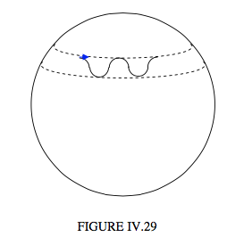
This motion corresponds to an initial condition in which you give the top an initial push in the forward direction as indicated by the little blue arrow. If the initial conditions are such that $\cos\alpha>\frac{L_{1}}{L_{3}}>\cos\beta$, the sign of $\dot{\phi}$ is different at the upper and lower bounds. Thus is illustrated in Figure IV.30

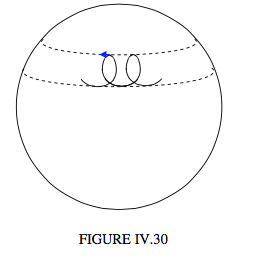
This motion would arise if you were initially to give a little backward push before letting go of the top, as indicated by the little blue arrow.

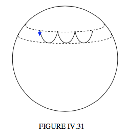
If the initial conditions are such that $L_{1}=L_{3}\cos\alpha$, then $\dot{\theta}$ and $\dot{\phi}$ are each zero at the upper bound of the nutation, and this was the situation in our numerical example. It corresponds to just letting the top drop when you let it go, without giving it either a forward or a backward push. This is illustrated in Figure IV.31.

As we discovered while doing our numerical example, the initial conditions $\dot{\theta} = \dot{\phi} = 0$ when $\theta = \alpha$ lead, in this third type of motion, to

$$\ L_{1} = L_{3} \cos \alpha \tag{4.10.20}\label{eq:4.10.20}$$

and

$$\ A = B \cos \alpha \tag{4.10.21}\label{eq:4.10.21}$$

In the case Equation $\ref{eq:4.10.13}$ becomes

$$\ \dot{\theta}^{2} = B(\cos \alpha - \cos \theta) - [\frac{L_{3}(\cos \alpha - \cos \theta)}{I_{1}\sin\theta}]^{2} \tag{4.10.22}\label{eq:4.10.22}$$

The lower bound to the nutation(i.e. how far the top falls) is found by putting $\theta = \beta$ when $\dot{\theta}$=0. This gives the following quadratic Equation for $\beta$:

$$\cos^{2}\beta - \frac{L^{2}_{3}}{I^{2}_{1} B} \cos\beta + \frac{L^{2}_{3}\cos \alpha}{I_{1} \sin \theta} \tag{4.10.23}\label{eq:4.10.23}$$

In our numerical example, this is

$$\cos^{2}\beta -7.725002 \cos \beta +5.690048 = 0, \tag{4.10.24}\label{eq:4.10.24}$$

which, naturally, has the same two solutions as we obtained when we solved the cubic Equation, namely 0.824 596 and 6.900 406.

Recalling the definition of B (Equation $\ref{eq:4.10.15}$), we see that Equation $\ref{eq:4.10.23}$ can be written

$$\ \cos \alpha - \cos\beta = \frac{2MglI_{1}}{L_{3}^{2}}\sin^{2}\beta, \tag{4.10.25}\label{eq:4.10.25}$$

from which we see that the greater $L_{3}$, the smaller the difference between $\alpha$ and $\beta$ - i.e. the smaller the amplitute of the nutation.

Equation $\ref{eq:4.10.12}$, with the help of Equations $\ref{eq:4.10.10}$ and $\ref{eq:4.10.11}$, can be written:

$$\ E - \frac{L^{2}_{3}}{2I_{3}}-\frac{1}{2}I_{1}\dot{\theta}^{2} = \frac{1}{2I_{1}}(L_{1}\csc\theta -L_{3} \cot \theta )^{2} + Mglcos\theta . \tag{4.10.26}\label{eq:4.10.26}$$

The left hand side is the total energy minus the spin and nutation kinetic energies. Thus the right hand side represents the effective potential energy $V_{e}(\theta)$ referred to a reference frame that is co-rotating with the precession. The term $Mgl\sin\theta$ needs no explanation. The negative of the derivative of the first term on the right hand side would be the “fictitious” force that “exists” in the corotating reference frame. The effective potential energy $V_{e}(\theta)$ is given by

$$\ \frac{V_{e}(\theta)}{L_{1}^{2}/(2I_{1})}=[\csc\theta- (L_{3}/L_{1})\cot\theta]^{2} + \frac{2I_{1}Mgl\cos\theta}{L_{1}^{2}}. \tag{4.10.27}\label{eq:4.10.27}$$

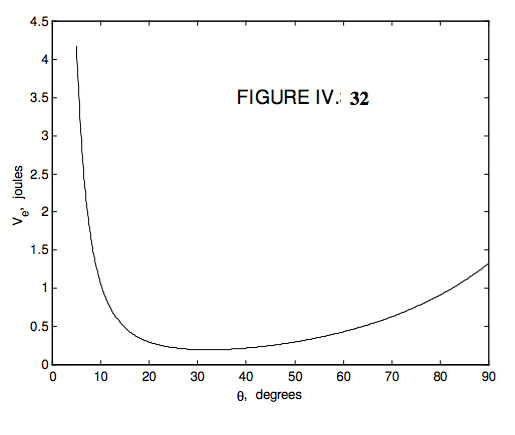
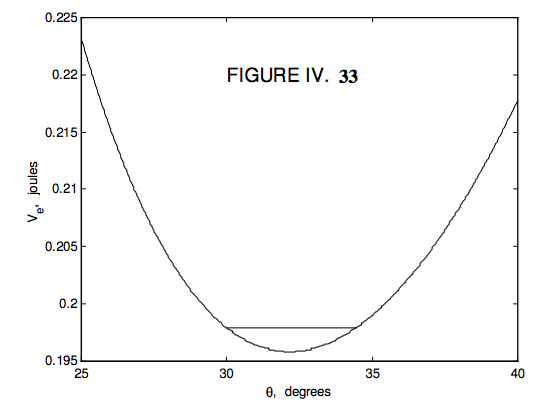
I draw $V_{e}(\theta)$ in Figures IV.32 and 33 using the values that we used in our numerical example – that is:

$$\ V_{e}(\theta) = 1.32081(\csc\theta - 1.154701\cot\theta)^{2} +0.229536\cos\theta \qquad \text{joules}. \tag{4.10.28}\label{eq:4.10.28}$$

Figure 32 is plotted up to 90° (although as mentioned earlier one could go further than this if the top were not spinning on a horizontal table), and Figure 33 is a close look close 2 to the minimum. One can see that if $E - L_{3}^{3}/(2I_{2}) = 0.1979$ the effective potential energy (which cannot go higher than this, and reaches this value only when ) $\dot{\theta}$ = 0 , the nutation limits are between 30° and 34° 24' . For a given $L_{3}$, for a larger total energy, the nutation limits are correspondingly wider. But for a given total energy, the larger the component $L_{3}$ of the angular momentum is, the lower will be the horizontal line and the narrower the nutation limits. If the top loses energy (e.g. because of air resistance, or friction at the point of contact with the table), the E = constant line will become lower 2 and lower, and the amplitude of the nutation will become less and less. If $E - L_{3}^{2}/(2I_{3})$ is equal to the minimum value of $V_{e}(\theta)$ there is only one solution for $\theta$, and there is no nutation. For energy less than this, there is no stationary value of $\theta$ and the top falls over.

We can find the rate of true regular precession quite simply as follows – and this is often done in introductory books.

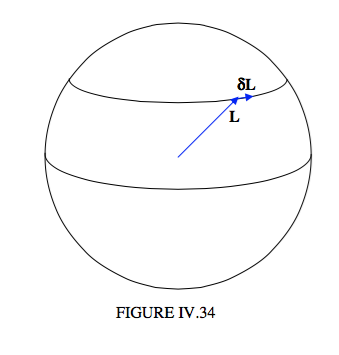
In Figure IV.34, the vector $\bf{L}$ represents the angular momentum at some time, and in a time interval $\delta t$ later the change in the angular momentum is $\boldsymbol\delta { \bf L}$. The angular momentum is changing because of the external torque, which is a horizontal vector of magnitude $Mgl\sin\theta$ (remind yourself from Figure XV .26 and 27). The rate of change of angular momentum is given by $\bf{L} = \tau$. In time $\delta t$ the tip of the vector $\bf{L}$ moves through a “distance” $\tau \delta t$. Denote by $\boldsymbol\Omega$ precessional angular velocity (the magnitude of which we have hitherto called $\dot{\phi}$). The tip of the angular momentum vector is moving in a small circle of radius $L\sin \theta$. We therefore see that $\tau = \Omega L \sin\theta$. Further, $\tau$ is perpendicular to both $\boldsymbol\Omega$ and $\bf{L}$. Therefore, in vector notation,

$$\boldsymbol\tau = \boldsymbol\Omega \times { \bf L} \tag{4.10.29}\label{eq:4.10.29}$$

Note that the magnitude of $\boldsymbol\tau$is $Mgl\sin\theta$ and the magnitude of $\boldsymbol\Omega \times \bf{L}$ is $\Omega L \sin\theta$, so that the rate of precession is

$$\ \Omega = \frac{Mgl}{L} \tag{4.10.30}\label{eq:4.10.30}$$

and is independent of $\theta$.
One can continue to analyse the motion of a top almost indefinitely, but there are two special cases that are perhaps worth noting and which I shall describe.

Special Case I. $L_{1} = L_{3}$.
In this case, Equation $\ref{eq:4.10.27}$ becomes

$$\ \frac{V_{e}(\theta)}{Mgl}= C(csc\theta - cot\theta)^{2} +\cos\theta \tag{4.10.31}\label{eq:4.10.31}$$

where

$$\ C = \frac{L_{1}^{2}}{2MglI_{1}} \tag{4.10.32}\label{eq:4.10.32}$$

It may be rather unlikely that $L_{1} = L_{3}$ exactly, but this case is of interest partly because it is exceptional in that $V_{e}(0)$ does not go to infinity; in fact $V_{e}(0)=Mgl$ whatever the value of $C$. Try substituting $\theta$ = 0 in Equation $\ref{eq:4.10.31}$ and see what you get! The right hand side is indeed 1, but you may have to work a little to get there. The other reason why this case is of interest is that it makes a useful introduction to case II, which is not impossibly unlikely, namely that $L_{1}$ is approximately equal to $L_{3}$, which leads to motion of some interest.

In Figure IV.35, I draw $\frac{V_{e}(0)}{Mgl}$ for several different $C$.

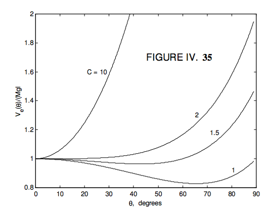
From the graphs, it looks as though, if $C \geq 2$, there is one equilibrium position, it is at $\theta$ = 0°(i.e. the top is vertical), and the equilibrium is stable, If $C < 2$, there are two equilibrium positions: the vertical position is unstable, and the other equilibrium position is stable. Thus if the top is spinning fast (large $C$) it can spin in the vertical position only (a “sleeping top”), but, as the top slows down owing to friction and air resistance, the vertical position will become unstable, and the top will fall down to a positive value of $\theta$.

These deductions are correct, for $\frac{dV_{e}}{d \theta} = 0$ results in

$$\ 2C(1-cos\theta)^{2} = \sin^{4}\theta \tag{4.10.33}\label{eq:4.10.33}$$

One solution is $\theta = 0$, and a second differentiation will show that this is stable or unstable according to whether $C$ is greater than or less than 2, although the second differentiation is slightly tedious, and it can be avoided. We can also note that $1 − \cos\theta$ is a common factor of the two sides of Equation $\ref{eq:4.10.33}$, and it can be divided out to yield a cubic Equation in $\cos\theta$:

$$\ 2C-1-(2C+1)\cos\theta -\cos^{2}\theta - \cos^{3}\theta =0, \tag{4.10.34}\label{eq:4.10.34}$$

which could be solved to find the second equilibrium point – but that again is slightly tedious. A less tedious way might be to take the square root of each side of Equation $\ref{eq:4.10.33}$:

$$\ \sqrt{2C}(1-\cos\theta)=1-\cos^{2}\theta \tag{4.10.35}\label{eq:4.10.35}$$

and then divide by the common factor (1 − \cos θ) to obtain

$$\cos \theta = \sqrt{2C} - 1, \tag{4.10.36}\label{eq:4.10.36}$$

which gives a real $\theta$ only if $C \geq 2$. Note also,if $C = \frac{1}{2}$, $\theta$ = 90° .

Special Case II. $L_{3} \approx L_{1}$.

In other words, $L_{1}$ and $L_{3}$ are not very different. In Figure IX.36 I draw $\frac{V_{e}(0)}{Mgl}$ for several different $C$, for $L_{3} = 1.01 L_{1}$.

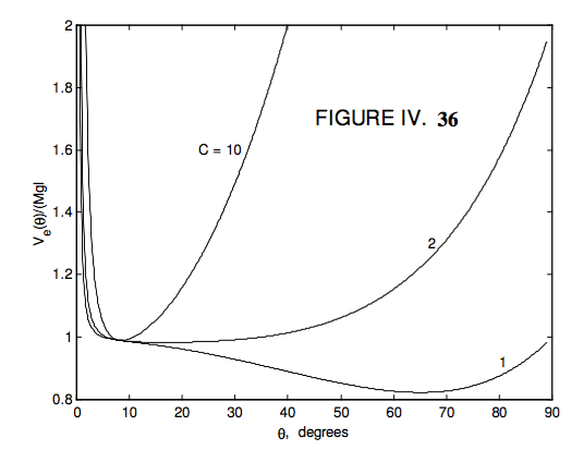
We see that for quite a large range of $C$ greater than 2 the stable equilibrium position is close to vertical. Even though the curve for $C = 2$ has a very broad minimum, the actual minimum is a little less than 17°. (I haven’t worked out the exact position – I’ll leave that to the reader.)