6.7: Helmholtz Coils

Let us calculate the field at a point halfway between two identical parallel plane coils. If the separation between the coils is equal to the radius of one of the coils, the arrangement is known as “Helmholtz coils”, and we shall see why they are of particular interest. To

begin with, however, we’ll start with two coils, each of radius $a$, separated by a distance $2c$.

There are $N$turns in each coil, and each carries a current $I$.

The field at $\text{P}$ is

$$B=\dfrac{\mu NIa^2}{2}\left ( \frac{1}{[a^2+(c-x)^2]^{3/2}}+\frac{1}{[a^2+(c+x)^2]^{3/2}}\right ) .\label{6.7.1}$$

At the origin $(x = 0)$, the field is

$$B=\dfrac{\mu NIa^2}{(a^2+c^2)^{3/2}}.$$

(What does this become if $c = 0$? Is this what you’d expect?)

If we express $B$ in units of $\mu NI/(2a)$ and $c$ and $x$ in units of $a$, Equation $\ref{6.7.1}$ becomes

$$B=\dfrac{1}{[1+(c-x)^2]^{3/2}}+\frac{1}{[1+(c+x)^2]^{3/2}}\label{6.7.4}.$$

Figure VI.7 shows the field as a function of $x$ for three values of $c$. The coil separation is $2c$, and distances are in units of the coil radius $a$. Notice that when $c= 0.5$, which means that the coil separation is equal to the coil radius, the field is uniform over a large range, and this is the usefulness of the Helmholtz arrangement for providing a uniform field. If you are energetic, you could try differentiating Equation $\ref{6.7.4}$ twice with respect to $x$ and show that the second derivative is zero when $c = 0.5$.

For the Helmholtz arrangement the field at the origin is

$$\frac{8\sqrt{5}}{25}\cdot \frac{\mu NI}{a}=\frac{0.7155 \mu NI}{a}.$$

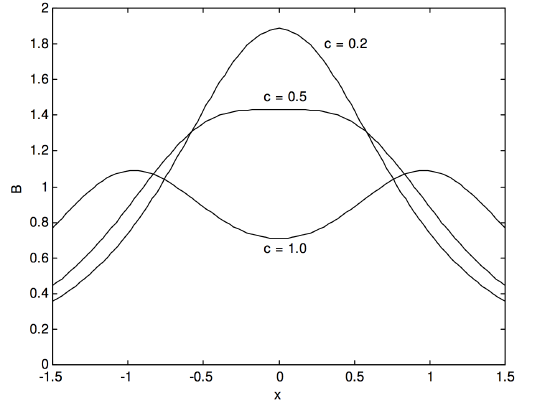
$\text{FIGURE VI.7}$