4.6: Second Law of Thermodynamics

Entropy

Up to this point in the course we have focused on conservation of energy which told us how the energy of the system changes when energy is transferred as heat or work in or out of the system, or how energy is transferred from one form to another within the same system. However, there are some physical phenomena that we took as given due to our knowledge of everyday experiences, rather than applying conservation of energy directly. For example, we have always assumed that heat will flow from the hot to the cold system. Imagine the opposite scenario of ice and warm water in an insulated container, where ice gets colder and the liquid gets warmer, each experiencing the same change in magnitude of thermal energy. Even though we know that this does not happen in nature, this process does not violate conservation of energy. Even more dramatically, we do not typically observe thermal energy converting to mechanical energies. Objects do not spontaneously cool off and leap into the air, loosing thermal energy and gaining potential energy. Although the reverse is a common process, in both cases conservation of energy again is not violated, Thus, we need something else to complete our understanding of energy, which we call entropy.

Macroscopic approach:

In the previous sections we defined work in terms of the energy transfer on an ideal gas as the integral of pressure over volume, \(W=-\int PdV\). Another form of energy transfer is heat, that we would also like to define in terms of an integral. Energy is transferred as work when there is a pressure difference between the system and its surroundings resulting in a change of volume. Energy is transferred as heat when there is a temperature difference, which then will result in a change of some extensive quantity (a quantity that depends on the size of the system, such as volume). For work this quantity was volume, for heat we call this quantity entropy, which is another state function. We arrive at an analogous equation for heat, in terms of an integral of temperature over entropy for a reversible process:

\[Q=\int TdS\label{entropy-int}\]

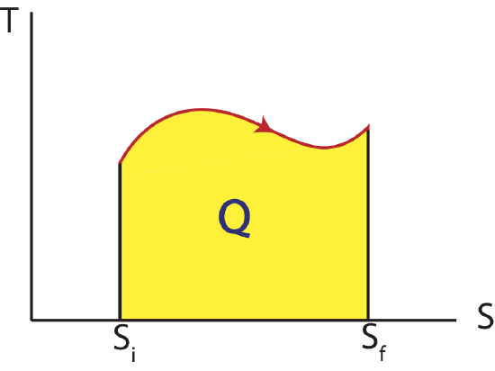
Thus, as we analyzed the work done in a process by calculating the area under a curve on a PV diagram, we can equivalently find the heat transfer by looking at the area under a curve on a TS diagram as shown below. As for PV diagram, another process that can be depicted on a state diagram must be quasi-static such that every point along the process between an initial and final state define the system as equilibrium.

Figure 4.3.1: Temperature vs Entropy, TS Diagram

In the case of heat the sign of the change in entropy is directly related to the sign of heat. Thus, when the entropy of the system is increasing, \(\Delta S >0\), heat is positive, \(Q>0\), and is flowing into the system. When the entropy of the system is decreasing, \(\Delta S <0\), heat is negative, \(Q<0\), and is flowing out the system.

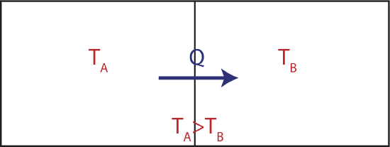
Now let us try to understand what heat that always flows from the hot to the cold system tells us about entropy. Consider two large thermal reservoirs exchanging heat. The meaning of a reservoir is that it is large enough to keep its temperature constant, even though heat can flow in and out of it as depicted in the figure below.

Figure 4.3.2: Two Reservoirs Exchanging Heat

If the two reservoirs depicted above define a close system, then the amount of heat that flowing into the colder reservoir at temperature \(T_B\) has to equal to the heat that was transferred out of the water reservoir at \(T_A\). If were were to depict this process on two TS diagrams, one for each reservoir, as seen below, the areas under the two curves have to equal since \(|Q_{in}|=|Q_{out}|\).

Figure 4.3.3: TS Diagrams for Two Reservoirs Exchanging Heat

The reservoir which is at a higher temperature, \(T_A\) will have a higher value on the y-axis with the processes going to the left, since heat is leaving. The lower temperature reservoir, \(T_B\), will have a lower value on the y-axis with the processes flowing to the right since the heat is entering this system. In order for the areas to be equal (the two yellow colored regions), the difference in entropy represented on the x-axis for higher temperature one has to be smaller than the the difference in entropy for the lower temperature one. In other words,

\[|S_{B,f}-S_{B,i}|>|S_{A,f}-S_{A,i}|\label{entropy-ext}\]

Note, the change in entropy that is positive for reservoir B is bigger in magnitude than the change that is negative for reservoir A. Assuming that entropy is additive like volume, \(S_{tot}=S_A+S_B\), the total change in entropy for this process is:

\[\Delta S_{tot}=\Delta S_A+\Delta S_B\]

Assuming the system consisting of reservoir A and B is closed and using the result from equation we arrive at a very important result from Equation \ref{entropy-ext}, known as the Second Law of Thermodynamics:

\[\Delta S_{tot}\geq 0\]

The entropy, S, of a closed system can never decrease in any process (the closed system could be a combined open system and the surroundings with which it interacts). If the process is reversible, the entropy of the closed system remains constant, \(\Delta S =0\). If the process is irreversible, the entropy of the closed system increases, \(\Delta S >0\).

We also arrive at another interpretation of the meaning of temperature. From the start of the course we have thought of temperature so far as a quantity that can be measured with a thermometer which then we defined as the indicator for thermal energy. The new definition comes from the discussion of heat and entropy. Another common form of writing Equation \ref{entropy-int} is:

\[\dfrac{1}{T}=\dfrac{\Delta S}{Q}\]

What the above equation tells us is that the slope of the entropy versus heat graph is the inverse of temperature. The higher the temperature the smaller the slope, since the slope is inversely proportional to temperature. This implies that entropy is changing at a slower rate as heat is transferred at higher temperatures and at a faster rate at lower temperatures. Since heat flows from hot to cold, the positive entropy change of the cold system will be greater in magnitude since it's at a lower temperature than the negative change of entropy in the warmer system. This again leads us to the Second Law of Thermodynamics assuring that the total change in entropy will always be positive.

Another way to write the equation for the change in entropy for a reversible process is:

\[\Delta S=\int \dfrac{dQ}{T}\]

When temperature is constant this simply becomes:

\[\Delta S=\dfrac{Q}{T}\]

When temperature is changing implying that there is no change in bond energy, using the definition for heat capacity we get:

\[\Delta S=C\int_{T_i}^{T_f} \dfrac{dT}{T}=C\ln\Big(\dfrac{T_f}{T_i}\Big)\]

The heat capacity depends on the type of process that is occurring.

Example \(\PageIndex{1}\)

You mix some of juice initially at 20°C with 0.2 kg of ice cubes. The ice cubes are initially at -5°C. You leave this in an open cup outside on a cold winter day and forget about it. After the system reached equilibrium, you return to get your juice, you find that 0.15kg of the ice cubes have melted. In this process the environment (cold winter outdoors) gained 100 J/K of entropy. You may treat juice as water.

Constants for water: \(c_{ice}=2.05 kJ/(kg K)\), \(c_{liq}=4.18 kJ/(kg K)\), \(\Delta H_{melt} = 334 kJ/kg\).

1. Find the mass of the juice.
2. Find the total change in entropy in this system.
3. Explain why this is an irreversible process and state what the reverse process would be in this scenario.

Solution

a) Since the system reached equilibrium and not all of the ice has melted, this implies that the equilibrium temperature is 0 ^oC. Using the 1^st Law of Thermodynamics we know that the change of energy of the ice, \(\Delta E_i\), and the juice, \(\Delta E_j\), must equal to the heat exchanged with the environment.

\[\Delta E_{j}+\Delta E_{i}=Q\nonumber\]

Since the final temperature is 0 ^oC, the juice just had a change of temperature from 20 ^oC to 0 ^oC, and the ice has a change in temperature from -5 ^oC to 0 ^oC, and then partially melted:

\[m_j c_{liq}\Delta T_{j}+m_i c_{sol}\Delta T_{i}+\Delta m_i\Delta H_{melt}=Q\nonumber\]

We can find \(Q\) that left the system for an environment that remains at constant temperature:

\[\Delta S_{env}=\frac{Q}{T}\nonumber\]

So,

\[Q=\Delta S_{env} T=(100 J/K)\times(273K)=27.3kJ\nonumber\]

This is the heat that entered the environment, thus -27.3 kJ left the system.

Solving for the mass of the juice from the above equation:

\[m_j =\frac{Q-m_i c_{sol}\Delta T_{i}-\Delta m_i\Delta H_{melt}}{c_{liq}\Delta T_{j}}=\frac{-27.3kJ-(0.2kg)\times(2.05kJ/kgK)\times(0+5)K-(0.15kg)\times(334 kJ/kg)}{(4.18 kJ/kgK)\times(0-20)K}=0.95kg\nonumber\]

b) The total change in entropy is the sum of all the changes:

\[\Delta S_{tot}=\Delta S_{i}+\Delta S_{j}+\Delta S_{env}\nonumber\]

For the ice:

\[\Delta S_i=m_ic_s\ln\Big(\frac{T_f}{T_i}\Big)+\frac{\Delta m_i\Delta H_{melt}}{T_{f}}=(0.2kg)\times(2.05kJ/kgK)\ln\Big(\frac{273}{268}\Big)+\frac{(0.15kg)\times(334 kJ/kg)}{273}=0.191 kJ/K\nonumber\]

For the juice:

\[\Delta S_i=m_jc_l\ln\Big(\frac{T_f}{T_i}\Big)=(0.95kg)\times(4.18kJ/kgK)\ln\Big(\frac{273}{293}\Big)=-0.281 kJ/K\nonumber\]

Therefore:

\[\Delta S_{tot}=0.191-0.281+0.10=10 J/K\nonumber\]

c) This process is irreversible because \(\Delta S_{tot}\geq 0\). The reverse process would be heat from the outside entering the cup, warming up the juice to 20°C, and freezing and cooling ice to -5°C. This is clearly not a likely event.

Microscopic approach:

Let us start with a brief overview of some simple statistics. The goal here is to understand the idea of equilibrium and to connect it to entropy from a statistical point of view using a model called Intro to Statistical Model of Thermodynamics. When describing an equilibrium state of a system, we can fully categorize it by measuring a few state functions, such as temperature, pressure, and volume. From a microscopic point of view these state function can be described by energies of the individual atoms or molecules that made up the system, such as the kinetic energy in three-dimensions of atoms in a monatomic gas. There are multiple ways that individual microscopic particles can have energies but still lead to the same values of state function, T, P, and V of the macroscopic system. It is exactly this multitude of microscopic states that lead to the same macroscopic state is related to entropy.

Let us start with a system which is simple to think about. Imagine you had a large box of an equal number blue and red balls, such that the probabilities of pulling out a blue or a red ball are equal. Every time you pull out a ball, you place it back in the box, so the number of blue and red always stays the same in the box. You want to analyze what is the most likely number of red balls you will have as you pull out more and more balls. Let us start with a simple situation of pulling out a ball two times. All the possible outcomes of our system are called microstates. When two balls taken from the box, there are a total of four microstates: RR, RB, BR, and BB, where "R" stands for red and "B" for blue. A macrostate is a possible macroscopic outcome that you can have typically described by multiple microstates, such as the number of red balls. In this case there are three possible macrostates: zero red balls, one red ball, and two red balls. We see that the probability of one red ball is the largest, since there are two microstates that describe the macrostate of one red ball. Since there is a total of four microstates, the probability of one red ball is 2/4 or 1/2. More generally, the probability of a macrostate \(s\) is the number of microstates of that state, \(\Omega_s\) divided by the total number of available microstates, \(\Omega_{tot}\) :

\[P_s=\dfrac{\Omega_s}{\Omega_{tot}}\]

We see from this equation that the most probably macrostate is the the one that has the most number of microstates. For an ideal gas, a microstate can be described by the locations of each atom in the gas and their corresponding kinetic energies in each dimension. A macrostate would be a specific temperature and pressure that the gas can have.

A summary of all the macrostates and the corresponding microstates for a four ball system is given the table below.

Macrostate	Microstate	Probability
0		\(\dfrac{1}{16}\)
1		\(\dfrac{1}{4}\)
2		\(\dfrac{3}{8}\)
3		\(\dfrac{1}{4}\)
4		\(\dfrac{1}{16}\)

We see from the four ball example that it is 6 times more likely to pull out 2 red balls than 4 red balls. As the number of balls that you pull out increases, so does the relative probability of half of them being red. For example, by counting microstates, you can calculate that for 100 balls, the probability of getting exactly half of them red is \(1\times 10^{29}\) times more than the probability of having all of them red. Moreover, having around half of them red (e.g. half plus or minus a few balls), is practically certain with near 100% probability. Thus, from the statistical point of view it becomes clear that for a macroscopically large system, there is a macrostate (in this example about half of the balls being red) which is much more likely than any other macrostate.

What does it mean for a system to evolve toward equilibrium? Statistically speaking the system will likely end up in a state which has the greatest number of microstates, since this is the most probable state. By definition we say that, equilibrium is the macrostate with the greatest number of microstates. Given enough time, any system will naturally evolve towards equilibrium.

There will always be some constraints limiting the number of microstates of a physical system composed of many particles. Some common examples of constraints are the available volume and total energy. Of course, either of these constraints could be relaxed, by increasing the volume, for example, or adding more energy to the system. But the point is, given whatever constraints actually exist, there is a total number of microstates that the system could find itself in. This total number of accessible microstates is usually represented with the uppercase Greek Omega, \(\Omega\).

\[S=k_B\ln\Omega\]

The number of microstates are not additive. We saw that when we pulled out 2 balls from the box, we found 4 number of microstates. For 4 balls, the number became 16, rather than 4+4=8. Thus, it appears that when systems are combined the number of microstates is multiplied:

\[\Omega_{total}=\Omega_1\times\Omega_2\]

This is exactly where the logarithm is helpful, since it turn entropy into an extensive (additive) state function, such as volume. It is clear that volume is extensive, if there was a partition in a container splitting it into individual volumes V1 and V₂, and then the partition was removed, the total volume would just equal to the sum of the individual ones, V_tot=V₁ +V₂. Entropy has the same extensive behavior which can be shown using properties of logarithmic functions:

\[S_{tot}=S_1+S_2=k_B\ln\Omega_1+k_B\ln\Omega_2=k_B\ln\Omega_1\times \Omega_2=k_B\ln\Omega_{tot}\]

Since the natural log increases with the number of microstates, entropy will also increase as the number of microstate increases. Since states with the most number of microstates are the most likely ones, entropy will always increase, arriving again at the Second Law of Thermodynamics, \(\Delta S\geq 0\) for a closed system.

Example \(\PageIndex{2}\)

Two quantum systems are brought into thermal contact allowing them to come to thermal equilibrium. Initially the hotter system has 10 accessible microstates, while the colder one has 4 accessible microstates. At equilibrium each system has the same number of microstates. Find the minimum number of microstates that each system can have at equilibrium.

Solution

The change in entropy of the warmer system, A, is:

\[\Delta S_{A}=\Delta S_{A,f}-\Delta S_{A,i}=k_B\ln\Omega_f-k_B\ln 10=k_B\ln\Big(\dfrac{\Omega_f}{10}\Big)\nonumber\]

The change in entropy of the colder system, B, is:

\[\Delta S_{B}=\Delta S_{B,f}-\Delta S_{B,i}=k_B\ln\Omega_f-k_B\ln 4=k_B\ln\Big(\dfrac{\Omega_f}{4}\Big)\nonumber\]

The total change in entropy is:

\[\Delta S_{tot}=\Delta S_{A}+\Delta S_{B}=k_B\ln\Big(\dfrac{\Omega_f}{10}\Big)+k_B\ln\Big(\dfrac{\Omega_f}{4}\Big)=k_B\ln\Big(\dfrac{\Omega_f}{10}\times\dfrac{\Omega_f}{4}\Big)=k_B\ln\Big(\dfrac{\Omega_f^2}{40}\Big)\nonumber\]

Second law states that \(\Delta S\geq 0\), resulting in

\[\Big(\dfrac{\Omega_f^2}{40}\Big)\geq 1\nonumber\]

or \(\Omega_f\geq\sqrt{40}\). Since the number of microstates has to be an integer and \(\sqrt{40}=6.32\), the minimum number of microstates that the equilibrium state must have is 7.