5.2: Measuring Ages - Lifetimes of Stars

What Do You Think: Burning and Stars

Advances in the understanding of radioactivity at the beginning of the 20th century enabled scientists to calculate the age of Earth accurately. However, the ages derived presented a problem to astronomers: they were not consistent with estimates of the age of the Sun.

Several decades earlier, the physicists William Thomson (Lord Kelvin) and Hermann von Helmholtz had attempted to estimate the Sun’s age. They made the assumption that the gravitational potential energy of the Sun was the source of energy that allowed it to shine. According to their model, as the Sun radiates energy from its surface, it should slowly contract, basically falling inward due to its own gravity. The contraction would provide the energy needed to keep the Sun hot and allow it to shine. (This is similar to the source of energy we tap into when we allow water to fall over a dam and then drive a turbine in an electrical generator.) However, the model gave a lifetime that was younger than the age of Earth, as detailed in Going Further 5.2: The Gravitational Lifetime of the Sun.

Another possible power source for the Sun that people once considered was combustion. Could it be that the Sun is just a big burning object, like a big piece of coal in the sky? That is what people did think a long time ago. We can put the idea to a test and see if it works, as you will do yourself in the activity The Chemical Lifetime of the Sun. Combustion is a type of chemical reaction, a process of combining a substance with oxygen in a way that produces a lot of energy. The typical energy in chemical bonds is about an electron-volt, or 1 eV (= 1.6 × 10^-19 joules in SI units). We are already familiar with these energy units from our explorations of light in the previous chapters. Even if we could assume that oxygen was available in the Sun to run the combustion reactions, the lifetime of the Sun derived from this method is even shorter than that of the gravitational method.

So, if neither gravity nor chemical burning is the source of energy for the Sun to shine, what is? That was a question that could not be answered by Kelvin or Helmholtz or by any other physicist or astronomer of the time. New physics was needed before a satisfactory understanding of the Sun could be found. By the start of the 20th century, scientists realized that some other, unknown form of energy must be powering the Sun. We have briefly touched on it: the physics of the atomic nucleus.

Calculating the Lifetime of the Sun

We can calculate the lifetime of the Sun (or any star) based on an analysis of its energetics. We determine how much total energy it has available, and then we compare that to the rate at which it is using its energy up. Mathematically, this can be expressed by the following equation that relates its power output, or luminsity (\(L\)), to its energy production.

\[L=\dfrac{E}{t}\nonumber \]

Luminosity (\(L\)), or power, in measured in watts and energy (\(E\)) in joules. The time (\(t\)) is in seconds. Recall that 1 watt = 1 joule/second.

If we rearrange the equation, we get:

\[t=\dfrac{E}{L}\nonumber \]

This means that the lifetime of the star depends on the total amount of energy (\(E\)) and the rate at which it is using that energy, which is the luminosity (\(L\)). If the luminosity is bigger, the lifetime will be shorter. An analogy for this would be driving your car until it runs out of gas: If you know how much gas is in the tank, and you know the rate at which your car uses gas, you can figure out when your car will run out of gas and stop moving.

To give you a better feel for the units of luminosity and energy, a typical compact fluorescent light bulb uses about 15 joules every second (for a 15-watt bulb), and a typical household might use about a thousand or so joules each second. A typical incandescent bulb is 60 watts. Keep these numbers in mind to compare to the luminosity of stars as we discuss them below.

The amount of energy that the Sun is emitting can be pretty easily measured at Earth’s surface. From that, we can deduce its total luminosity. Measurements have shown that there is about 1.4 kW of solar energy striking each square meter of Earth’s surface (on the daylight side). This value is an average and varies with cloud cover, time of day, latitude, and things like that. Nonetheless, if we had a square meter of material and held it facing the Sun at the distance of Earth’s orbit, it would have about 1.4 kW of solar radiation striking it. Of course, the Sun is not sending energy only through the 1 square meter that we measure. It is sending that amount of energy through every square meter on a sphere that completely surrounds it and has a radius equal to Earth's orbital radius, 1AU. To figure out how many square meters there are surrounding the Sun on a sphere with a radius the size of Earth’s orbit, we use geometry. We know that the area of a sphere is given by:

\[A=4πR^2\nonumber \]

Since the radius of Earth’s orbit is about 150 million km, or 1.5 × 10¹¹ m, the area will be: 4\(\pi\)(1.5 × 10¹¹ m)² = 2.8 × 10²³ m². Since each of these square meters has about 1.4 kJ of energy passing through it every second, the Sun must be emitting about (2.8 × 10²³ m²) × (1400 W/m²) = 4 × 10²⁶ W from its entire surface (i.e, in all directions). This is known as the solar luminosity—in other words, the Sun produces 4 × 10²⁶ J each second that it shines.

So, is a particular energy source enough to power the Sun for billions of years? We know how much energy the Sun emits every second. We also now know how much energy the Sun contains, both in terms of chemical and gravitational energy. With these numbers, we can estimate how many seconds the Sun can continue to shine.

GOING FURTHER 5.2: THE GRAVITATIONAL LIFETIME OF THE SUN

GOING FURTHER 5.3: WHY THE GRAVITATIONAL LIFETIME CANNOT BE FIXED

The Chemical Lifetime of the Sun

Long ago, people thought the Sun was just a big burning object on fire, like a big piece of coal in the sky. We can put that idea to a physics test and see if it works.

Combustion is a type of oxidation, a process of combining a substance with oxygen. There are other ways to oxidize materials, but combustion produces a lot of energy. The typical energy in chemical bonds is about an electron-volt, or 1 eV. We are already familiar with these energy units from our discussion of light in the previous chapters. However, electron-volts are not convenient for our purposes here. We should use joules; 1 eV = 1.602 × 10^-19 J.

Now assume that we have oxygen available in the Sun to run the combustion reactions. We now know that is not true, but certainly no one knew that prior to the turn of the 20th century. In the activity below, we will assume that the Sun is entirely made of oxygen, and when one oxygen atom combusts, an electron-volt of energy is released.

1. The atomic mass of oxygen is 16, and the mass of a proton (or a neutron) is about 1.67 × 10^-27 kg. What is the mass of oxygen in kg?

 

kg

Show your work:

 

2. Assuming that all the mass of the Sun is in the form of oxygen atoms, and that the mass of the Sun is 2 × 10³⁰ kg, use your answer from part 1 to figure out how many atoms of oxygen could be in the Sun.

 

atoms

Show your work:

 

3. Assuming that burning 1 oxygen atom releases 1 eV of energy, how much total energy would be available from combustion of all the atoms of oxygen in the Sun (from question 2)? Express your answer in joules.

 

joules

Show your work:

 

4. The Sun’s luminosity is 4 × 10²⁶ W. Use this luminosity to compute the time it will take for all of the available combustion energy (from question 3) to be used up. Express your answer in years.

 

years Show your work:

 

5. From this estimate of the chemical combustion lifetime of the Sun (from question 4), can combustion be the source of the Sun’s energy?

Yes

No

Explain your reasoning:

 

The Nuclear Lifetime of the Sun

We have seen how certain atomic nuclei undergo decays that convert one nucleus to a different one. It turns out to be possible to make those reactions run the other direction. Of course, the right physical conditions are required for the inverse decays to happen. Still other nuclear processes are possible, ones involving only stable nuclei. All of these processes go under the general name of nuclear reactions, and they play a vital role in the Sun and other stars.

There were many scientific advances between the time the study of radioactivity was undertaken and a workable theory of solar energy production was put forward. One of the most important of these was the realization that the Sun is composed almost entirely of hydrogen and helium. Small amounts of heavier elements are also present, but together they make up only about 2% of the mass of the Sun. This discovery was made by Cecelia Payne-Gaposchkin and presented as her doctoral dissertation in astrophysics at Radcliffe College, now part of Harvard University, in 1925. Payne-Gaposchkin used the then-nascent field of quantum mechanics to reach what was a very startling conclusion for the time. Her thesis is still considered by many to be the greatest Ph.D. dissertation ever done in the field of astrophysics.

Another important discovery bearing on solar energy production had been made 20 years earlier. Published in 1905 under the title Zur Elektrodynamik bewegter Körper (On the Electrodynamics of Moving Bodies) by Albert Einstein, at the time a clerk in the patent office of Bern, Switzerland, the paper made the astounding claim (one among several) that mass and energy are interconvertible. Many other advances were relevant as well, but we will explore how these two ideas impacted the understanding of the workings of the Sun and other stars.

As a starting point, consider the alpha particle, ⁴He. We introduced this particle earlier during our discussion of radioactivity. The alpha particle is the most common isotope of helium. It is composed of two protons and two neutrons. The masses of these particles are shown in Table 5.2.

Table 5.2

PARTICLE	PROTON	NEUTRON	2 PROTONS + 2 NEUTRONS	ALPHA (MEASURED)	DIFFERENCE
Mass (10^-^27kg)	1.672621637	1.674927211	6.695097696	6.64465620	0.050441496

If we add up the masses of the protons and the neutrons that make up the alpha particle, we find that the alpha particle has a mass lower than its constituent parts. This addition has been done in the table, with the difference being given in the last column. The difference is small, only about 0.7%. Still, how can it be that the protons and neutrons have lower mass when collected into an alpha particle than they do when out on their own? This difference is known as the binding energy, and it relates directly to mass-energy interconversion. Some of the mass of the protons and neutrons is converted to energy in creating an alpha particle, and that energy is released to the environment when the alpha particle is formed. The amount of energy is given by Einstein’s famous mass-energy equivalence.

\[E=mc^2\nonumber \]

where \(E\) = energy, \(m\) = mass, and \(c\) = the speed of light.

This energy release presents a possible source of energy for the Sun. As was shown by Cecelia Payne-Gaposchkin, the vast majority of the Sun is hydrogen; most of the rest is helium. Perhaps the Sun derives its energy by converting the hydrogen to helium and extracting energy in the process. The general nuclear reaction would be the conversion, in net, of four protons to an alpha particle.

\[\ce{4p→ ^4He}\nonumber \]

This type of nuclear reaction, where lighter elements combine to form heavier elements, is known as nuclear fusion. These are distinct from reactions in which heavier elements split apart into lighter ones in nuclear fission.

GOING FURTHER 5.4: NUCLEAR REACTIONS IN THE SUN AND OTHER STARS

Energy of Hydrogen Fusion

1. Using the information in Table 5.2, find the difference in mass (in kg) between the helium nucleus and the four protons.

 

kg Show your work:

 

2. How much energy does this mass correspond to in J? Hints: use Einstein's famous equation E=mc². The speed of light is about 3 x 10⁸ m/s.

 

J

3. How much energy does this correspond to in eV?

 

eV

Show your work:

 

In the previous activity, you should have found that energy could be extracted if we could devise a way to change four protons into a helium nucleus. We will save the discussion of how that might occur for later. For now, you will find the nuclear energy lifetime of the Sun and see if it is consistent with the Sun's lifetime of at least 5 billion years or so - the approximate age of Earth.

Nuclear Energy Lifetime for the Sun

In this activity, you will estimate the amount of time that the Sun could exist if it were being powered by the conversion of hydrogen to helium through nuclear fusion reactions. In the nuclear reactions we are considering, one kind of atom (hydrogen) is being converted into another (helium). Follow these steps to work through the activity:

1. Recall that the mass of the Sun is 2 × 10³⁰ kg. Assuming that all the mass in the Sun is hydrogen, and remembering that hydrogen is just a single proton (of mass 1.67 × 10^-27 kg), how many hydrogen atoms are in the Sun?

 

atoms

2. Recall that it takes 4 protons (hydrogen atoms) for each nuclear reaction. How many reactions will the Sun be able to produce?

 

reactions

3. Given the number of reactions (from question 2) and the energy (in joules) produced in each reaction (that you calculated in the activity of Energy of Hydrogen Fusion), how much total energy is produced?

 

J

4. Now you will find the lifetime. Use the total nuclear energy available that you just calculated and the luminosity of the Sun, which is 4 × 10²⁶ W. Express your final answer for the nuclear lifetime in years.

 

years Show your work:

 

5. Is nuclear energy generation a viable way for the Sun to produce its energy given what we know about the age of the Earth?

 

6. Is this still the case, even if only 1/10th of the mass of the Sun ever undergoes nuclear reactions?

 

In this case, what value do you get for the lifetime of the Sun (in billions of years)?

 

billion years

 

Lifetimes of Stars Other Than the Sun

The models of hydrogen fusion are the processes that set the basic timescale for stellar lifetimes. However, there is one other aspect of nuclear fusion that we have not really touched upon: the rate at which the hydrogen fusion takes place depends on the temperature and density of the gas. And not just in a small way. The nuclear reaction rate in the process used by low-mass stars like the Sun (see Going Further 5.4: Nuclear Reactions in the Sun and Other Stars) depends on the temperature to about the fourth power! That means if the temperature doubles, say, from 10 million to 20 million degrees, the nuclear reaction rate goes up by a factor of 2⁴. That is a factor of 16, so a star with twice the Sun’s temperature would run through its fuel 16 times faster.

The interesting part of all this is that more massive stars must have higher internal pressure to support themselves against their own weight (see Going Further 5.3: Why the Gravitational Lifetime Cannot Be Fixed). More internal pressure means they must be hotter, and hotter means that they run through their fuel faster. To make things even more extreme, the most massive stars do not produce their energy via the same chain of processes as low-mass stars (see Going Further 5.4: Nuclear Reactions in the Sun and Other Stars). In high-mass stars, the temperature dependence is more like T¹⁵. For these reactions, doubling the temperature increases the fusion rate by more than a factor of 10,000! As a result, even though massive stars have more fuel, they last much less time than low-mass stars because they go through their mass so much more quickly.

To make an analogy with cars, low-mass stars are like hatchbacks: they have smaller gas tanks but run through it less quickly so they can run for a long time; high-mass stars are like SUVs: they have bigger gas tanks, but run through their fuel so quickly that it is not long before they run out.

LIFETIMES AND LUMINOSITIES OF STARS WITH DIFFERENT MASSES

In this activity, you will explore the relationships among the masses, luminosities, and lifetimes for stars that are fusing hydrogen.

A. Predictions: lifetime and mass

1. How do you think a star’s lifetime will depend on its mass?

If star A is twice as massive as star B, it will have a lifetime that is two times longer.

If star A is twice as massive as star B, it will have a lifetime that is half as long.

If star A is twice as massive as star B, it will have a lifetime that is more than two times longer.

If star A is twice as massive as star B, it will have a lifetime that is less than half as long.

Even if star A is twice as massive as star B, mass does not matter; they will have the same lifetime.

Now watch the animation, which shows how much time it takes for stars to end their main sequence lifetimes. (More massive stars are depicted as larger in size.)

Play Activity

2. Resolve any discrepancies with your predictions.

 

3. What additional information do you need to fully test your predictions?

B. Examining lifetime, mass, and luminosity

Next, click on the stars to further examine their properties, such as mass, luminosity, and lifetime. To look for more stars, click and drag with the mouse inside the window to move around.

Play Activity

1. Now you can fully test your predictions. Choose one star from your data set and another star with approximately twice its mass. How do their lifetimes compare? Resolve any discrepancies with your predictions.

 

2. How does the lifetime of a star with 5 times the mass of the Sun compare to that of the Sun?

 

3. Based on your answers to the above questions, how do you think the nuclear fusion rate for a high mass star is greater than, less than, or the same as that of a low mass star?

 

4. Now we will graph the data to determine the general trends and relationships. You can toggle between “plot” mode and “starfield” mode by clicking the appropriate buttons. To add more stars to the data set, go to starfield mode and click on them (click on a star again to remove it).

a. In the plot mode, use the pull-down menus to select mass on the x-axis and lifetime of the y-axis. What does this plot tell you about how a star’s lifetime depends on its mass?

 

b. Now compare the curve options to your data. What type of relationship fits mass and lifetime the best?

 

c. In the plot mode, use the pull-down menus to select mass on the x-axis and luminosity on the y-axis. What does this plot tell you about how a star’s luminosity depends on its mass?

 

d. Now compare the curve options to your data. What type of relationship fits mass and luminosity the best?

 

e. If a star A is twice as massive as star B, how will its luminosity compare?

 

5. Summarize the relationships among mass, lifetime, luminosity, and nuclear fusion rate for a main sequence star.

 

There is a mathematical relation that describes the tendency of more massive stars to use their fuel more quickly. It turns out that the luminosity of a star is roughly proportional to its mass raised to the third power.

\[L\sim M^3\nonumber \]

The luminosity, \(L\), thus increases rapidly with mass, \(M\).

The actual relationship is a bit more complicated, with the exponent being closer to 2.5 for stars with masses similar to the Sun’s or lower. For much more massive stars, the exponent is more like 3.5. Still, we can use this mass–luminosity relationship to explore, somewhat crudely, the typical lifetimes of stars.

We know that the lifetime of a star should be roughly given by the ratio of the amount of fuel it has to the rate at which it uses up that fuel. This is how we estimated the lifetime for the Sun previously. So, we can write as follows.

\[t∼\dfrac{M}{L}\nonumber \]

Using the mass–luminosity relation, we can combine these expressions. We then have the relation below.

\[t∼\dfrac{M}{M^3}=\dfrac{1}{M^2}\nonumber \]

So, we should expect that the more massive a star, the shorter its lifetime. The effect is dramatic. More massive stars live much shorter lives. A star with a mass 10 times that of the Sun will live roughly 1% as long. On the other hand, a star with a mass only 1/10th the Sun’s mass will live about 100 times longer.

We thus expect that any stars that have ever formed over the history of the Universe to still be around if they have masses 1/10th the mass of the Sun. In contrast, stars 10 to 100 times the mass of the Sun last for only a few million years. This is such a short period of time that they should not even be able to leave the sites of star formation where they are born before they run out of fuel.

Though these are only rough estimates, they still give us a general idea of stellar lifetimes. To compute the actual lifetimes for a given star, we have to use sophisticated computer models that take into account not only the star’s mass, but also things like composition. The models also use great care to compute nuclear reaction rates, energy transport, and more. However, those details turn out not to make a huge difference in the lifetimes. Our simple estimates still give us good ballpark figures. They also produce approximately the correct trends of stellar lifetime with mass.

Comparing the Lifetimes of Stars With Different Masses

Worked Example:

1. The Sun’s lifetime is about 10 billion years. Estimate the lifetime of a star with twice the mass of the Sun.

• Given: The ratio of the masses is 2:1
• Concept: The lifetime goes as the inverse square of the mass: t ~ 1/M²
• Solve: So to find the ratio of the lifetimes, take the inverse square of the ratio of masses: t ~ 1/(2/1)² = ¼
• So, for a star with twice the mass of the Sun, its lifetime would be one-quarter that of the Sun, or ¼ × 10 billion years = 2.5 billion years.

Questions:

1. Use the relation for stellar lifetimes to estimate the lifetime of a star with ½ the mass of the Sun

 

years

which is

 

billion years

Stellar Properties and the H-r Diagram 

On a perfectly clear evening far away from city lights, you would only be able to see about 3,000 stars. Within 10 light-years of Earth, there are only 12 stars, including our Sun. Yet, beyond those that we can see with our naked eyes, we have found that there are hundreds of billions of stars in our Galaxy alone.

You might have noticed that not all stars appear the same. Looking up at night, a careful viewing shows that some stars are slightly more red or blue or yellow than others. Early astronomers noticed these color differences too, but a true understanding of stars did not begin until the 19th century. That is when astronomers began to employ the new tools of spectroscopy and photography, and these allowed them to begin to study the stars’ properties in detail. The application of photography and spectroscopy to astronomy in the late 19th century marks the birth of the modern science of astrophysics.

Using the new spectral methods, astronomers created a classification scheme for the stars based on patterns of lines seen in their spectra. Stellar spectral classification was first based upon the presence or absence of four prominent spectral absorption features: those from hydrogen, those from calcium and sodium, those from molecules, and those from carbon. This scheme, developed by the Italian astronomer and Catholic priest Angelo Secchi (1818–1878) in the 1860s, was taken up and expanded upon by Edward Pickering (1846–1919) and his “computers,” a group of female astronomy researchers at the Harvard College Observatory. These investigations started in the 1880s, and they quickly developed into the most advanced set of stellar observations in the world.

Wilhemina Fleming (1857–1911) was one of the Harvard computers, and she was tasked with making sense of stellar spectra. She subdivided each of Secchi’s classes into subclasses and gave them letter designations, A through Q. These were based upon more refined differences in their spectra that had become apparent from the superior data that were being collected by the Harvard observers. Another of the computers, Antonia Maury (1866–1952), then took up the work. She rearranged the ordering of some of Fleming’s letter classes and also replaced the letter classification system with one based upon numbers. Her system was quite detailed, but also complicated. It did not find much favor with her colleagues at the Observatory because it was difficult to understand and use. Finally, in 1901, Annie Jump Cannon (1863-1941) took up the challenge. She greatly simplified the spectral classification system of Maury. She also returned to letter classes, like Fleming, but with far fewer class designations in total. She mostly retained the ordering of Maury while reordering a few additional spectral types herself. Each of these revisions of spectral classification was based on the increasingly more detailed measurements of the spectral features of stars. Cannon’s basic system of stellar classes is the one still in use today.

There are seven primary categories in the classification system created by Annie Cannon. They are O, B, A, F, G, K, and M. Cannon further divided these into subclasses, so that a B5 star would be midway between a B and an A star, an A2 would be partway from A to F, etc. In 1925, Cecelia Payne-Gaposchkin, whom we have already mentioned, showed that the spectral types are related to temperature, but that discovery depended upon the development of the quantum theory of the atom. Some of the properties of the stellar types are shown in Table 5.3.

Table 5.3: Stellar Properties and Spectral Classification

SPECTRAL CLASS	COLOR	TEMPERATURE (K)	MASS (SOLAR UNITS*)	RADIUS (SOLAR UNITS*)
O	Blue	>3.0 × 10^4	>16	>6.6
B	Blue white	1.0 × 10^4 – 3.0 × 10^4	2.1 – 16	1.8 – 6.6
A	White, bluish white	7.5 × 10^3 – 1.0 × 10^4	1.4 – 2.1	1.4 – 1.8
F	White, yellowish white	6.0 × 10^3 – 7.5 × 10^3	1.0 – 1.4	1.2 – 1.4
G	Yellow	5.2 × 10^3 – 6.0 × 10^3	0.8 – 1.0	1.0 – 1.2
K	Orange	3.7 × 10^3 – 5.2 × 10^3	0.5 – 0.8	0.7 – 1.0
M	Red	<3.7 × 10^3	0.1 – 0.5	< 0.7
*The units of mass and radius in the table are solar masses and solar radii. One solar mass is equal to the mass of our Sun (about 2 × 10^30 kg), and one solar radius is equal to the radius of our Sun (about 7 × 10^5 km).

While the computers of Harvard College Observatory busied themselves classifying stars (and doing other things), other astronomers were searching for different patterns in stellar properties. In 1911, Ejnar Hertzsprung (1873–1967), in Denmark, plotted stellar luminosity against stellar color. He measured the “color” of each star using its brightness measured in two filters, centered at different wavelengths of light, and comparing them. Two years later, the American astronomer Henry Norris Russell (1877–1957) independently plotted a star’s brightness against its spectral class. Because both spectral class and color are different ways of characterizing the star’s temperature, these two relationships are really the same thing. Hertzsprung and Russell discovered this relationship independently but nearly simultaneously. And so plots of stellar brightness vs. temperature are now called Hertzsprung-Russell diagrams, or just H-R diagrams, to honor the astronomers who first made them (Figure 5.3).

Figure 5.3: The Hertzsprung-Russell diagram shows the relationship between a star’s temperature, spectral class, luminosity, and absolute magnitude. Notice that high temperatures are on the left, corresponding to spectral class O, and lower temperatures are on the right, corresponding to spectral class M. Brighter stars are toward the top of the diagram and dimmer stars are toward the bottom. Credit: NASA/SSU/Aurore Simmonet.

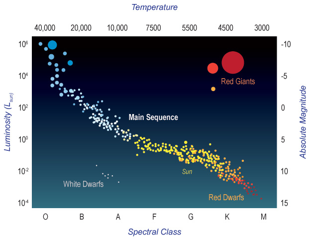
The majority of stars lie along a central diagonal line in the diagram, called the main sequence. Main-sequence stars are in the main part of their lifetimes, fusing hydrogen into helium. During this steady hydrogen-burning phase, the stars are in a state of hydrostatic equilibrium. This means that the gravitational pressure pushing inward and compressing them is balanced by outward thermal pressure. The stars are stable because any tendency of the star to compress will heat its interior, thereby increasing the nuclear fusion rate, releasing more energy, and thus increasing the pressure. The increased pressure then overcomes the compression and expands the star. On the other hand, any tendency of the star to expand will cool the star, thereby slowing the nuclear reaction rate. The reduced reaction rate means lower energy production and further lowering the temperature and, thus, pressure. The reduced pressure then allows gravity to compress the star. So any departure from equilibrium causes effects that return the system to the original steady state: These negative feedback creates a stable equilibrium condition that lasts as long as the star has nuclear fuel to fuse in its core.

In a sense, a star is a giant self-regulating thermostat. It adjusts itself so that it maintains just enough nuclear fusion to create pressure to support itself against gravity, but not so much that it blows itself apart. Again, this is true as long as there is fuel in the core for fusion to occur.

On the H-R diagram, as one goes from the red to the blue-white stars on the main sequence, the stars not only become brighter but they also become hotter and more massive. Color, temperature, mass, and radius are all intrinsically linked for main sequence stars. This is due to the physics involved.

As stars age, they run out of hydrogen to fuse, and this causes them to adjust their internal structure. They evolve off the main sequence and occupy different regions of the H-R diagram. Some of these changes will be described in Section 3.6, on stellar evolution.

Examining clusters of stars plotted on the H-R diagram gives us an additional way to determine the ages of objects in the Universe. We can estimate the ages of star clusters because all stars in the cluster started forming at the same epoch from the same parent cloud. By looking at which stars have ceased hydrogen fusion and which ones have not, we can estimate the age of the cluster.

Using such plots, we have learned that the oldest parts of our galaxy are around 13 billion years old, nearly as old as the Universe itself. We have also learned that there are very young parts of the Galaxy, some even in the process of forming. There are objects with intermediate ages as well. You will determine the ages of several star clusters in the next activity.

Star Clusters and Stellar Lifetimes

The plots shown here are for three different star clusters. Along the horizontal axis is the star’s surface temperature, with lower temperatures on the right and higher temperatures on the left. The vertical axis is the star’s brightness, with dimmer on the bottom and brighter at the top. Brightness is given in terms of apparent visual magnitude (see Going Further 3.6: The Magnitude System).

Figure A.1: The Hertzsprung-Russell diagrams for three different open clusters. Credit: NASA/SSU/Aurore Simmonet.

Notice that all of the star clusters plotted show a line of stars running from the lower right to upper left. We will ignore stars that are not along this line for the time being.

1. Do you expect the stars at the left of each graph to have low masses or high masses? Explain your reasoning.

 

2. Given your answer in question 1, should these stars have long lifetimes or short lifetimes?

 

3. Assuming that all the stars in a given cluster were formed around the same time, does the plot make sense, given your answers in questions 1 and 2? Explain how it either does or does not.

 

4. If you can, list the clusters from youngest to oldest. Explain your reasoning.