10.5: The Source of Gravity

What Do You Think: Where Does Gravity Come From?

In the descriptions of gravity we have looked at so far, we have left off one important part: What is the source of spacetime curvature? We have described what curvature is, at least in a basic sense, and we have described how curvature affects the motion of particles and the perceptions of space and time that different observers have. But where does the curvature actually come from?

This is like asking where the force of gravity comes from in Newtonian theory. Newton had a ready answer: from masses. Newton’s law of gravitation describes precisely what the gravitational force between two point masses will be, given their separation. In Newton’s view, gravity comes from the interaction between the two masses (and not from either of the masses by themselves). What is the corresponding law in general relativity?

It turns out that it is possible to write down a precise mathematical relationship in general relativity, akin to Newton’s law of gravitation, but the meaning of the relation is not as easy to convey. We will write it down, and you will see why: The so-called Einstein equation can be written as:

\[\textbf{G}=\dfrac{8\pi G}{c^4}\textbf{T} \nonumber \]

This expression is not very revealing, so we will break it down a bit. The capital G on the right is the familiar gravitational constant from Newton’s law, c⁴ is the speed of light (raised to the fourth power). The 8 and \(\pi\) are numbers, of course. It is hard to understand how this simple expression leads to spacetime curvature, but that is because we are hiding a lot.

The G and T terms actually stand for fairly complicated mathematical entities known as tensors. That is why we have written them in boldface; we want them to stand out to convey that they are not just normal numbers. G is an object that describes the four-dimensional spacetime curvature. T describes the four-dimensional mass–energy distribution. This deceptively simple expression is actually 10 independent equations relating the curvature to the mass–energy distribution. In a similar way, Newton’s gravitational law is actually three equations that describe the gravitational forces in the independent x, y, and z directions, but we generally write it as a single equation involving the 3-dimensional force and position vectors. The Einstein equation is something like that, but it describes a more complicated view of gravitation than can be conveyed in just a single (or three!) equation.

Solving the 10 equations contained in the Einstein equation produces the spacetime interval for that particular distribution of mass–energy. For a spherically symmetric, time-independent mass–energy distribution we get the spacetime interval we saw earlier in the chapter. We have already discussed how that describes gravity around Earth and the Sun. It also describes the spacetime around black holes. For other mass–energy distributions we get different curvature described by different spacetime intervals. (See Going Further 10.7: The Einstein Equation for more details.)

Because the mathematics required to solve the Einstein equation are advanced, we have not shown you an example of how this is done. Even the simplest example requires math beyond the level assumed for this unit. However, we did not want to leave our discussion of general relativity without at least giving you a brief description of the connection between mass–energy, the source of gravity, and spacetime curvature, the way gravity gets expressed.

As in Newtonian gravity, the source of gravitational effects in general relativity is mass. However, in general relativity, other forms of energy produce a gravitational effect too, even the energy in gravity itself. That is why we have been careful to say “mass–energy” when discussing the source part of the Einstein equation. This should not be surprising if you recall the mass–energy equivalence from special relativity.

\[E = mc^2 \nonumber \]

General relativity carries over this equivalence from special relativity, as it does many other ideas. But in general relativity we are not limited to inertial frames, where any motion must be unchanging. In general relativity, which was initially intended to be a mere expansion into accelerated motion, what we have found is a radical new way of describing the gravitational interaction that underlies the dynamics of the Universe on large scales. In later chapters we will see that the general relativistic view of gravity leads to truly astounding notions regarding the origin and evolution of the cosmos.

Going Further 10.7: the Einstein Equation

We have just been introduced to two terms: the four-dimensional spacetime curvature, G_μν, and the four-dimensional mass–energy distribution, T_μν. How can we visualize these terms to try to gain a deeper understanding of what they represent?

We introduced the concept of a vector when we discussed velocity, and we went into more detail when we discussed forces. A vector is a physical quantity that has both strength and direction. We can specify its components in the three spatial dimensions: x, y, and z. By specifying the sizes of these components, we also specify the direction that the force vector is pointing.

For example:

• F_grav = (10,0,0) indicates a force with strength of 10 N in the x-direction
• F_grav = (10,10,0) indicates a force with strength = (10² + 10²)^1/2 = 14.14 N at an angle 45 degrees between the x and y axes.
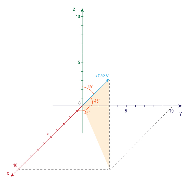
• F_grav = (10,10,10) indicates a force with strength = (10² + 10² + 10²)^1/2 = 17.32 N at an angle 45 degrees between the x and y axes and also 45 degrees between the x–y plane and the z-axis.

These force vectors are illustrated in Figure B.8.7.

Figure B.8.7: (a) A force vector with magnitude 10 N in the x-direction; (b) a force vector with magnitude 14.14 N at an angle 45 degrees between the x- and y-axes; and (c) a force vector with magnitude 17.3 N at an angle 45 degrees between the x- and y-axes and also 45 degrees between the x-y plane and the z-axis. Credit: NASA/Sonoma State/A. Simonnet

Vectors are useful mathematical tools. They can express forces that point in one particular direction. However, when we use vectors to represent (for example) the gravitational force, we are also assuming that the objects that are being affected can be treated as points. That is to say, we assume they are very, very small, so that the force can act on the objects as though all their mass was concentrated at one tiny point. Furthermore, we can describe the location of any point by its coordinates in three-dimensional space.

But what if we have really large objects? For example, Earth is rather large compared to satellites that are in orbit around it. So approximating the satellites as tiny points compared to Earth works pretty well. (However, as we have seen in our discussion of GPS, there are errors that arise that need to be corrected, which are about 1 part in one billion.) But Earth is not that much larger than the Moon, and both have bulges and craters. We might therefore expect that neither one of these objects looks like a tiny point to the other. Instead, we need to consider the entire Earth–Moon system when we do an accurate calculation of how they affect one another.

In these types of situations, we cannot describe the gravitational force as acting in a specific, linear three-dimensional direction. Instead, we need to specify the components of the gravitational acceleration acting in different directions in four-dimensional spacetime. Then we can account for the curvature correctly. The four-dimensional spacetime curvature G, which has components, \(G_{μν}\), is the mathematical way that we express this more complicated situation. Rather than being a series of three numbers (like a vector), it can be represented mathematically by a special type of 4 × 4 matrix called a tensor.

This is how the components of \(G_{μν}\) are defined:

\[ G_{\mu\nu}= \begin{pmatrix} g_{11}& g_{12}& g_{13}& g_{14} \\ g_{21}& g_{22}& g_{23}& g_{24} \\ g_{31}& g_{32}& g_{33}& g_{34} \\ g_{41}& g_{42}& g_{43}& g_{44} \end{pmatrix} \nonumber \]

In this case, the diagonal components of the matrix appear in the expression for curvature that we defined previously:

\[ s^2= g_{11}\left(\Delta x\right)^2 + g_{22}\left(\Delta y\right)^2 + g_{33}\left(\Delta z\right)^2 - g_{44}\left(c\Delta t\right)^2 \nonumber \]

For special relativity in flat space, the components (g₁₁, g₂₂, g₃₃, g₄₄) = (1,1,1,–1) yielding the familiar expression for the spacetime interval:

\[ s^2=\left(\Delta x\right)^2+\left(\Delta y\right)^2 + \left(\Delta z\right)^2-\left(c\Delta t\right)^2 \nonumber \]

The matter-energy tensor, T, which has components \(T_{\mu\nu}\)_, is a similar 4 × 4 matrix that describes the field associated with the distribution of the matter and energy in spacetime.

\[ T_{\mu\nu}= \begin{pmatrix} T_{11}& T_{12}& T_{13}& T_{14} \\ T_{21}& T_{22}& T_{23}& T_{24} \\ T_{31}& T_{32}& T_{33}& T_{34} \\ T_{41}& T_{42}& T_{43}& T_{44} \end{pmatrix} \nonumber \]

To be clear, the individual matrix elements in G and T each describe some aspect of local curvature, in the case of G, or the local mass-energy content, for T. Putting both of these tensors together into Einstein’s equation leads to a series of 10 independent equations - there would be more, but certain symmetries reduce the total number to 10. These equations must be solved simultaneously in order to correctly calculate the gravitational effect (spacetime curvature) created by the corresponding mass-energy distribution. In a few simple cases, these equations can be solved with pencil and paper; however, in all other cases, the solution requires numerical calculations by supercomputers.