12.2: Lensing by Point Masses

Learning Objectives

• You will understand how the lensing effect depends on the relative positions of the source, lens and observer.
• You will understand that the mass of the lens can be determined using gravitational lensing.
• You will understand that objects such as dim stars, brown dwarfs, and stellar remnants (white dwarfs, neutron stars, black holes) can act as gravitational lenses. Collectively they are called MACHOs.
• You will understand that microlensing observations imply that a large percentage of the dark matter in our Galactic halo is not regular matter (MACHOs) but rather a yet-to-be-determined exotic form of matter.

What Do You Think: Microlensing

Modeling Gravitational Lenses

Gravitational lenses are easiest to understand if we employ a simple model, similar to the one used to understand conventional lenses in optical systems. We assume that the light travels in a straight line until it reaches the lens, and then its direction is altered by some angle. After that the light travels in a straight line to the observer. The lens itself is assumed to be infinitely thin and to act on the light only as it crosses the plane of the lens. This model captures the essential behavior of the lens system: the lens causes the source to appear to be displaced from the point of view of the observer. At the same time, it avoids the complicated mathematical treatment needed to find the actual path of the light through the region of strong gravity that creates the lens in the first place.

The assumptions used for all lenses, including gravitational ones, are the following:

1. Light travels in a straight line from the source to the infinitely thin lens.
2. The light is bent at the lens plane (and only at the lens plane).
3. The light then travels in a straight line to the observer.

Students who are familiar with the geometrical approach to optics or who have read Going Further 12.1: Optical Lenses will see some similarities between these assumptions and those used in the treatment of glass lenses. The geometry of a lens system is shown in Figure 12.2. A source located at point S is emitting light that is deflected by a lens located between the source and some observer, located at point O. The lens could be anything with mass: a star or planet, or a galaxy or cluster of galaxies. If the lens did not deflect the light, then the observer would see the source at its true position. However, due to the deflection of the light caused by the lens’s gravity, the image of the source is observed to be at position I.

Figure 12.2 The figure shows a side view of the basic elements of a gravitational lens system. The observer is at point O, the source is at S. These two are separated by a distance D_SO . The angle α is equal to the deflection angle. The deflection of the light makes the image appear to be at position I as seen by the observer. The image has thus been offset by a small amount compared to the source, i.e. the case if no lens were present. The angle θ is the angular separation of the image from the observer. The lens is taken to be somewhere along the path of the light a distance D_LO from the observer and D_LS from the source. These two distances do not have to be the same. Credit: NASA/SSU /Aurore Simonnet

In Figure 12.2, the line connecting the observer to the lens is called the optical axis. We can imagine the optical axis extending behind the lens indefinitely. The source can be located on the optical axis, but in general it does not have to be. That is why we have located the point S slightly off the optical axis. Since gravity always bends a light ray toward the optical axis, the position of the image, point I, will always be located farther from the optical axis than the actual source of the light for the configuration shown. There is an additional image formed below the optical axis for which this is not true, but we will consider that image later. The distance between the source and the observer is D_SO, the distance between the lens and the observer is D_LO, and the distance between the lens and the source is D_LS. The angle θ in Figure 12.2 is the angular separation between the observer, the image, and the optical axis.

In Going Further 12.2: The Lens Equation, we examine the geometry of gravitational lenses in more detail, and derive a general equation relating the angles and distances for several cases.

It turns out that if the source, lens, and observer are all lined up along the optical axis, the image of the lensed object makes a ring around the lens, as shown in Figure 12.3. The ring-like image is called an Einstein ring.

Figure 12.3 This object (known as SDSS J073728.45+321618.5) is one of several Einstein rings discovered as part of the Sloan Lens ACS Survey (SLACS). The width of this image is about 8 arcsec. For more information, see the press release. Credit: NASA, ESA, A. Bolton (Harvard-Smithsonian CfA) and the SLACS Team

The angular radius, θ_E, of an Einstein ring is given below.

\[\theta_E=\sqrt{\left (\frac{4GM}{c^2} \right ) \left ( \frac{D_{LS}}{D_{LO}D_{SO}}\right )} \nonumber \]

This is called the Einstein radius of the lens system. We distinguish it by adding the subscript E to the angle θ from Figure 12.2. As usual, G and c are the gravitational constant and the speed of light. The size of the Einstein ring varies only with the geometry of the lens, as expressed inside the parentheses on the right-hand side, and on the total projected mass within the impact parameter, M(b). For example, if the mass within the impact parameter is larger, then θ_E will be larger. If the distance between the source and observer (D_SO) is bigger, then θ_E will be smaller.

The following activities will give you an idea of the size of the Einstein radius for objects with masses relevant to astrophysics.

The Einstein Radius

In this activity, you will be able to adjust the parameters in the lens equation in order to determine their effect on the size of the Einstein ring.

There are three sliders, one for each of the following:

• The mass of the lens (M)
• The distance to the source from the observer (D_SO)
• The relative positioning of lens, source, and observer (the ratio D_LS/D_LO)

Play Activity

A. Mass of the Lens

1.

2. 3.

4.

B. Distance to the Source from the Observer

1.

2. I 3. 4.

C. Relative Position of the Lens

1.

2.

Size of the Einstein Radius

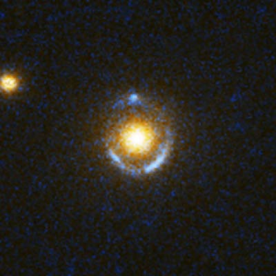
In this activity, we will compute the sizes of Einstein radii for solar mass lenses in our Galaxy as well as for extragalactic lenses like the one pictured in Figure 12.4.

Worked Examples:

1. Compute the Einstein radius for a distant galaxy being lensed by a foreground trillion solar mass galaxy. Assume that all of the mass of the lens lies within the impact parameter, b. Assume the distance to the gravitational lens is 1000 Mpc and the distance between the lens and source is 2000 Mpc.

• Given: Mass M = 1e12 × 2e30 kg = 2e42 kg, D_LS = 2000 Mpc, D_LO = 1000 Mpc
• Given: Mass \(M = 10^{12}\times 2\times 10^{30}\,{\rm kg}=2\times 10^{42}\,{\rm kg}\), D_LS = 2000 Mpc, D_LO = 1000 Mpc
• Find: θ_E, the Einstein radius in radians and arcseconds
• Concept(s):

\(\theta_E=\sqrt{\left (\frac{4GM}{c^2} \right ) \left ( \frac{D_{LS}}{D_{LO}D_{SO}}\right )}\)

• where \(c = 3\times 10^8\, {\rm m/s}\) and \(1\, {\rm Mpc} = 3.09\times 19^{22}\, {\rm m}\)
  and D_SO = D_LS + D_LO
• Solution:

First, get the distances in SI units

(meters):
D_LS = 2000 Mpc x (3.09E22 m / 1 Mpc) = 6.18E25 m
D_LO = 1000 Mpc x (3.09E22 m / 1 Mpc) = 3.09E25 m
D_SO = D_LS + D_LO = 3000 Mpc x (3.09E22 m / 1 Mpc) = 9.27E25 m

Now we can plug the numbers in to get θ_E:

\(\theta_E = \sqrt{\left (\frac{(4)(6.67\times 19^{-11}\,{\rm N\,m^2\,kg^{-2}})(2\times 10^{42}\,{\rm kg})}{(3\times 10^8\, {\rm m/s})^2}\right ) \left ( \frac{6.18\times 10^{25}\,{\rm m}}{(3.09\times 10^{25}\,{\rm m})(9.27\times 10^{25}\,{\rm m})}\right )}\)

\(=1.13\times 10^{-5}\,{\rm radian}\)

• Now express this angle in arcseconds. The conversion factor for radians to arcseconds is: 1 radian = 2.06E5 arcseconds.
• θ_E = (1.13E-5 radians)(2.06E5 arcseconds / radian) = 2.3 arcseconds.

To see how to compute the Einstein radius for a solar mass object in our galaxy, see Math Exploration 12.1.

Math Exploration 12.1

Questions:

1.

Determining the Mass of a Lens

In this activity, you will analyze gravitationally lensed images to determine the mass of the lens.

Worked Example:

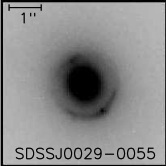
1. The image in Figure A.12.1 is an Einstein ring from the SLACS survey.

Figure A.12.1 This object, SDSS J0029-0055, is one of the Einstein rings discovered as part of the Sloan Lens ACS Survey (SLACS). Credit: Adapted from Bolton et al. (2008), Astrophysical Journal, 682, 964

In their paper, the SLACS team has determined that the radius of the Einstein ring is 1.11 arcsec, the distance

to the source is 9.67 × 10²⁵ m, and the distance to the lens is 2.84 × 10²⁵ m. Based on this information, what is the mass of the lens?

• Given: θ_E = 1.11 arcsec, D_SO = 9.67E25 m, D_LO = 2.84E25 m
• Find: M, the mass of the lens
• Concept(s):

\(\theta_E=\sqrt{\left (\frac{4GM}{c^2} \right ) \left ( \frac{D_{LS}}{D_{LO}D_{SO}}\right )}\)

where \(c = 3\times 10^8\, {\rm m/s}\) and \(1\, {\rm Mpc} = 3.09\times 10^{22}\, {\rm m}\) and D_SO = D_LS + D_LO

• Solution:

First, get the distance between the lens and the source: D_LS = D_SO - D_LO = 9.67E25 m - 2.84E25 m = 6.83E25 m

We will also need the Einstein radius in radians: θ_E = 1.11 arcsec × (1 radian / 2.05E5 arcsec) = 5.39E-6 radians

Now rearrange the equation to solve for M.

\(M = \left ( \frac{(\theta_Ec)^2}{4G} \right ) \left ( \frac{D_{LO}D_{SO}}{D_{LS}} \right )\)

Plugging in numbers, we get the solution.

\(M = \left ( \frac{ [(5.39\times 10^{-6})(3\times 10^8\, {\rm m/s}) ]^2}{(4)(6.67\times 10^{=11}\, {\rm N\,m^2\,kg^{-2}})} \right ) \left ( \frac{(2.84\times 10^{25}\, {\rm m})(9.67\times 10^{25}\, {\rm m})}{6.83\times 10^{25}\, {\rm m}} \right ) = 3.94\times 10^{41}\, {\rm kg}\)

We can express this in solar masses if we divide by 2E30 kg.

\(M = 1.97\times 10^{11}\) solar masses

Questions

1.

2.

In the previous activities you saw how changing the geometry or mass of the lens changed the size of the Einstein ring. However, in all cases you might have noticed that the ring is extremely small. For typical Galactic lenses the Einstein radius is only a few milli-arcseconds, too small to be seen. For extragalactic lenses the size is larger, though still usually less than an arcsecond.

GOING FURTHER 12.2: THE LENS EQUATION

Microlensing

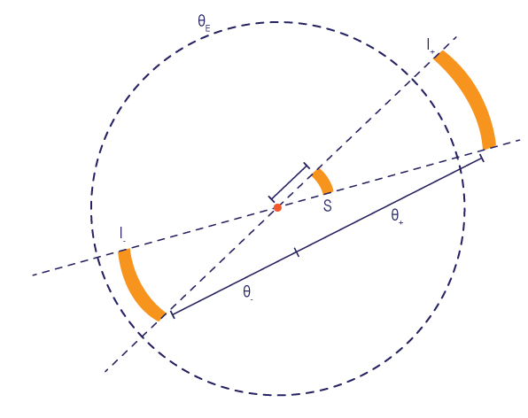
The simplest mass distribution for a gravitational lens is that of a point mass, which creates two images, one on each side of the optical axis. When the lens, source, and observer line up we have the case of the last section, an Einstein ring. The images are distorted into arcs that completely encircle the lens.

However, if the source is moved off the optical axis, then the images separate. One, which we will call \(\theta_-\), moves inward toward the optical axis. This is the image that we mentioned, but ignored in Figure 12.2 earlier; it “passes under” the optical axis. The other image, which we will call \(\theta_+\), the one shown in Figure 12.2, moves outward. See Figure 12.4 for an illustration.

Figure 12.4 A point-mass gravitational lens will create two images of a source. In these diagrams, the gravitational lens is depicted as a small red dot and the source is shown as a blue spiral galaxy . The diagrams are drawn from the viewpoint of an observer looking at the sky. (a) If the source lies directly behind the lens, then the images overlap on the Einstein ring, as shown at left. (b) If the source is offset slightly, as on the right, then the images separate, one lying inside the Einstein ring (θ_- ), the other lying outside it (θ₊ ). Credit: NASA/SSU /Aurore Simonnet

The following activity allows you to explore how gravitational lensing will modify the appearance of an image as the angle between the source and lens is adjusted.

Lensing by a Point Mass

In this activity, you will use an interactive diagram that provides a simulated view through a telescope of a source object that has been lensed by a point mass. When the source object lies directly behind a massive lens, it is possible to have it lensed such that the image forms a ring running entirely around the lens, which might or might not itself be visible. The simulation in the activity lets you change the alignment of the lens and source and then see how the images formed by the lens change.

Play Activity

The simulation begins with a perfect alignment between the source, lens, and observer. The lens is a point mass, represented by a white dot, the source is a larger blue disk in the center of the screen. Because of the perfect alignment, the image is a ring, shown in blue.

Use the slider to move the source slightly off the center of the optical axis. The image will change as you do this.

Move the source farther to the left and right. You should notice that the image changes more dramatically as you move the source farther from the center.

1. 2. 3. 4. 5.

6.

7. 8.

In Section 12.2.1, we saw an HST picture of an extragalactic Einstein ring, but calculated that the sizes of Einstein rings due to lensing events within our Galaxy would be too small too see. Because of the tiny size of the images produced, this kind of lensing is called microlensing. However, the small size of microlensing does not mean that its effects are not measurable.

In addition to being displaced, you may have noticed in the previous activity that the images are also magnified in size compared to the source. For a spherically symmetric lens, the image on the outside of the Einstein ring (θ₊) is larger than the one on the inside of the Einstein ring (θ_-). The greater the distance off of the center of the optical axis the source is, the smaller both images will be. If the source is at an angular separation from the lens that is greater than the Einstein radius, the θ_- will be smaller than the source; the farther away, the smaller, until eventually no lensing effect is seen.

These changes in size turn out to be extremely useful. Because gravitational lenses preserve the surface brightness of the source in the images it produces, if the image is larger than the source it also becomes brighter. On the other hand, if the image becomes smaller than the source, then the image is dimmer because it has a smaller area.

Even if we cannot see the individual images, we can detect the changes in brightness caused by the lens; a gravitational microlensing event will cause the brightness of the source to appear to increase over what it would be without lensing. Figure 12.5 illustrates this effect.

Figure 12.5 A point-mass lens changes the size of the images relative to the source. Because the lensing effect preserves surface brightness, a larger image will be brighter than the source. Credit: NASA/SSU/Aurore Simonnet

In Figure 12.5, we see schematically how the images produced in a lens will increase the source's apparent brightness when the images are too close to each other to be resolved. In that case they look like a single image. For an observer, the brightness of the individual images combine to create an apparent brightness that is the sum of the two. This magnification is due only to the fact that the images each have the same surface brightness as the source, while being larger in area. The magnification for a point-mass lens (like a star, for example) is given by the expression that follows.

\[m = \frac{1}{1- \left (\frac{\theta_E}{\theta}\right )^4} \nonumber \]

When θ is smaller than the Einstein radius (the θ_- case), the magnification is negative, meaning that the image of the source is inverted (upside down). That is not important for a point source, but it is important when we consider lensing of extended sources like galaxies. When the angle θ is larger than the Einstein radius (the θ₊ case), the magnification is positive, so the image is right-side up relative to the source. In the next exercise, you will plot the magnification as a function of θ and use your plot to draw some conclusions about the brightness of a lensed source.

Magnification by a Point Source

1.

2.

3.

4.

5.

Of course, the brightness of an image in a lens with static geometry does not change, and whether it is dimmer or brighter than the source alone cannot be determined. However, if the geometry is not static, in other words, if the angular separation between the lens and source changes in time, then the source will vary in brightness with time. In real life, we cannot control the geometry of astrophysical lenses the way we did in the previous interactive activity. However, sometimes naturally occurring motions will change the geometry for us. This effect was first suggested as a means to look for non-luminous objects in our Galaxy by the Polish astrophysicist Bohdan Paczyński (1940–2007) in the mid-1980s.

Paczyński proposed to monitor millions of stars in the Large Magellanic Cloud (LMC), a small satellite galaxy of the Milky Way, and wait for a massive object (a lens) to pass in front of one of them as it orbited through the halo of the Milky Way (see Figure 12.6). The possible lensing objects in our Galactic halo could be: dim stars, large planets, brown dwarfs, black holes, neutron stars, or white dwarfs. Together these objects are known as MACHOs, for Massive Astrophysical Compact Halo Objects.

The resulting change in brightness of the background LMC star as it was lensed would reveal the presence of the otherwise invisible lens object, the MACHO, in our halo. A chance alignment of a background star with a foreground lens is extremely rare. However, by increasing the number of background stars - by observing the relatively dense stellar field of the LMC - the likelihood grows. That is exactly the advantage gained by monitoring an object like the LMC.

The LMC lies outside the disk of our Galaxy at a distance slightly over 160,000 light-years. Its distance makes it a promising target for microlensing surveys, first, because its stellar density on the sky is increased by its distance and, second, because a sightline to the LMC passes through a large part of our Galaxy’s halo. In addition, the LMC is close enough to cover a large fraction of the sky, at least compared to other galaxies. Because of all these favorable properties, Paczyński reasoned that the LMC would make a good candidate for finding microlensing events. In practice, astronomers realized that the Small Magellanic Cloud (SMC) and even the Galactic bulge would also be suitable targets for microlensing surveys.

Figure 12.6 (a) Light from a star in the Large Magellanic Cloud (LMC) is lensed by an unseen object in the halo of our Galaxy. (Note: LMC and lens not to scale in this drawing.) (b) The LMC is the largest known of several dozen small galaxies that orbit the Milky Way. The LMC and another satellite, the Small Magellanic Cloud, are easily visible from the southern hemisphere, though they are too far south to be seen from most of the northern hemisphere. Credit: (a) NASA/SSU /Aurore Simonnet , (b) upload.wikimedia.org/wikipedi ...arp.750pix.jpg

One complication with Pacyński’s strategy is that microlensing is not the only process that can cause a star’s brightness to vary. Many stars are inherently variable. We have already discussed the Cepheid variable stars in Chapter 4, but many other types of variable stars exist. Fortunately, they can all be distinguished from microlensing events. For instance, variable stars often show periodic variations (Cepheids being just one example), whereas microlensing of a star will be extremely unlikely to repeat. For other kinds of variable stars, the color of the star changes with its brightness due to a changing surface temperature— novae and supernovae exhibit this kind of behavior. Microlensing, like all gravitational lensing, behaves the same in all wavelengths of light. So in a microlensing event the color of the source will not appear to change over the course of the brightening. In addition, the brightening and dimming phases in a microlensing event should by symmetric in time. That is not the case with other transient astrophysical sources. A model light curve for a microlensing event is shown in Figure 12.7.

Figure 12.7 Gravitational microlensing events are distinct from other sorts of variable sources because they are perfectly symmetric in time, rising and falling in precisely the same manner. In addition, the brightening and dimming is the same at all wavelengths, which is not the case for most other variable astrophysical sources. Finally, the brightening will not repeat; it is a one-time event. Credit: NASA/SSU/Aurore Simonnet

Several microlensing surveys were undertaken through the 1990s, two of them of fairly large scale. The first of these was the Polish OGLE project, led by Pacyński and Andrezj Udalski of the University of Warsaw. OGLE (Optical Gravitational Lensing Experiment) has been running since 1992 and, as of this writing (2021), is still in operation. Observational data are collected with a dedicated 1-meter telescope at Las Campanas Observatory in Northern Chile. It has used wide-field imaging to monitor many hundreds of millions of stars in the Galactic bulge and the LMC and SMC. Another large project, started about a year after OGLE, was called the MACHO Project, which ran until 1999. The MACHO Project was a collaboration between astronomers at Mt. Stromlo and Siding Springs Observatories in Australia, and teams from several campuses of the University of California and the Lawrence Livermore National Laboratory in the United States. Like OGLE, the MACHO Project surveyed stars in the Galactic bulge and the LMC and SMC. Other projects were also undertaken over the past two decades to monitor the LMC, SMC, and Galactic bulge for gravitational microlensing events. Light curves from several microlensing events are shown in Figure 12.8.

Figure 12.8 Light curves (flux vs. time) for three microlensing events. The MACHO team observed these events by monitoring 8.6 million stars in the LMC for a little over a year. Each event shows the same signature in red and blue light, as expected from microlensing, but not other potential sources of variability. Credit: NASA/SSU/Aurore Simonnet. Adapted from Alcock et al. (1995) Physical Review Letters, 74, 286

The upshot of all these projects is that massive objects like white dwarfs, neutron stars, black holes, and brown dwarfs—the most likely kinds of objects to be MACHOs—cannot make up more than half of (much less all of) the dark matter of our Galaxy’s halo. There are simply too few microlensing events. Still, MACHOs do seem to account for a significant fraction of the dark matter in the Galaxy’s halo, most likely around 20%. This means that at least half of the dark matter must be made of some sort of exotic matter, and the most likely amount is about 80%. From the MACHO surveys we know that most of the dark matter in galaxies is not composed of neutrons, protons, and electrons, the stuff of familiar matter. It is made of some form of matter still to be discovered.

The following activity allows you to explore how a MACHO’s mass, velocity, and impact parameter influence a gravitational microlensing light curve.

MACHOs

In this activity, you will manipulate the mass, impact parameter, and velocity of a MACHO to determine how each of these variables affects the light curve observed when the MACHO lenses a distant star.

A peak in the light curve is created when the lensing MACHO passes in front of the star, causing the starlight to be magnified.

Play Activity

1. 2. 3. 4. 5. 6. 7.