15.3: Observations of Variations in the CMB

Learning Objectives

• You will understand what the spots are on CMB anisotropy maps
• You will understand how CMB measurements are made

What Do You Think: Variations in the CMB

When scientists look at the spatial distribution of the CMB in detail, they notice that superimposed on the nearly uniform background are tiny (about 10 – 100 parts per million) variations in temperature. This departure from uniformity, called anisotropy, was first observed by the Differential Microwave Radiometer (DMR) instrument on the COBE satellite in 1991 (Figure 15.6). This was important because for the first time it showed that the microwave background was not completely even. Since COBE’s early result, fluctuations in the CMB have been measured with increasing precision by dozens of instruments.

Figure 15.2 such that the red spots are slightly hotter than the blue spots by about 1/10,000th of a degree Kelvin.Animated Figure 15.7 shows a map of the CMB as observed by COBE and then later by the WMAP satellite at better resolution . It is possible to distinguish smaller angular sizes in the WMAP data . The red spots in the map correspond to slightly hotter regions and the blue spots correspond to cooler regions. The contrast between the hotter and colder regions is greatly exaggerated in order to see the effect; their typical temperature differences are about 1/10,000th of a degree!

Animated Figure 15.7 CMB anisotropy was first observed by the COBE satellite in 1991 at large angular scales (initial image in animation). Since then, it has been observed with better resolution by dozens of other instruments, including the WMAP satellite (final image in animation). The contrast has been enhanced compared to the CMB map in Figure 15.2 such that the red spots are slightly hotter than the blue spots by about 1/10,000th of a degree Kelvin. The WMAP image has better angular resolution than the COBE/DMR image. The difference between DMR and WMAP is similar to the difference between a near-sighted person without their glasses and a person who does not need glasses trying to recognize faces in a crowded room. The person who does not need glasses can see more detail than the person who does. Credit: NASA/WMAP Science Team

In both COBE and WMAP data, microwave signals from our Galaxy and other galaxies have been removed from the map, leaving only an image of the CMB. This is possible because the CMB has a unique blackbody spectral signature. Other sources of microwave emission, such as dust in our galaxy, have different spectral signatures. By observing the sky at several different frequencies, we are able to isolate and then subtract the sources other than the CMB. This process is illustrated in Animated Figure 15.8, with data from the Planck satellite.

Animated Figure 15.8 Microwave radiation from our Galaxy and other galaxies has been removed from the data in order to make a map of only the CMB. Credit: ESA and the Planck Collaboration

Another source of microwave light that can be found in CMB maps is a signature from the interaction of CMB photons with galaxy clusters, known as the Sunyaev-Zel’dovich (SZ) effect. Because of observations of the SZ effect, we know the CMB must be cosmological, that is, coming from all over the Universe, not just a nearby source (such as our Galaxy). Light from the CMB is distorted in the vicinity of galaxy clusters, which means it must be coming from places beyond the galaxy clusters (which are themselves far away) in order to be affected. The SZ effect can be seen at great distances, because it does not follow an inverse square law. This makes it ideal for finding galaxy clusters. Several groups are involved in efforts to measure the SZ effect and use it to survey galaxy clusters, as described in Going Further 15.1: The Sunyaev-Zel’dovich (SZ) Effect.

Going Further 15.1: The Sunyaev-Zel’dovich Effect

The Sunyaev-Zel’dovich effect is caused by interactions of photons with charged particles. We have already discussed on several occasions how photons can be scattered by charged particles, typically electrons. Sometimes this scattering merely changes the direction of the photons without changing their energy. That is what happens to sunlight as it passes through Earth’s atmosphere, and the preferential scattering of short wavelengths over longer causes the sky to appear blue on a clear day.

However, it is also possible for the scattering of light to transfer energy to or from the photons. If the population of scattering electrons has on average more energy than the population of photons, then energy is transferred to the photons, which appear hotter as a result. On the other hand, if the typical energy of the electrons is lower than the energy of the photons, then the light will transfer energy to the electrons. The light cools at it looses energy to the electrons.

The microwave background began as light with a typical temperature around 3000K. Since the Universe has grown by a factor of about a thousand since the CMB was created, the CMB light now is characterized by a temperature of around 3K, and of course, it was cooling from 3000K to 3K over its entire journey. However, some of the microwave photons have encountered galaxy clusters as they traveled through the cosmos. These photons have had their temperature modified by the scattering described previously.

In addition to containing galaxies, galaxy clusters also contain immense amounts of hot gas. The gas, which actually dominates the total baryonic mass of the clusters, has a temperature around 10 million kelvin, much higher than that of the CMB. This is because it sits deep in the gravitational well of the cluster. When CMB photons encounter the hot gas they gain energy from its particles because the CMB is so much cooler than the typical electron in the cluster gas. As a result, the photons passing through a cluster have a slightly increased temperature than CMB photons that don’t pass through a cluster. The spectrum is distorted and shifted to higher energy. The CMB photons mark the positions of the clusters on the sky because they cause the clusters to stand out as small spots in the microwave background. At higher wavelengths than the peak of the CMB, these spots are hotter, and at longer wavelengths (lower energies), these spots are colder, because the photons that would normally be present have been shifted to a different part of the spectrum. An example of an SZ cluster observation is shown in Figure B.15.1.

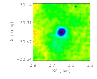
FIGURE B.15.1: SZ EFFECT. Galaxy cluster Abell 2744 as seen by the South Pole Telescope (SPT). Light from the CMB interacts with the hot gas in the cluster, causing a cold spot at the wavelengths that SPT observes. This is called the Sunyaev-Zel’dovich (SZ) effect. Credit: SPT Collaboration.

The SZ effect is important at high-l values, or small angular scales, because galaxy clusters are not very large on the sky. The small SZ temperature fluctuations are not caused by any primordial cosmological parameters, they are modifications of the original CMB spectrum by intervening mass concentrations as its photons travel to us. These fluctuations must be accounted for in the cosmological analysis of the CMB since they introduce a spurious signal (or noise, if you prefer) on the true cosmological perturbations.

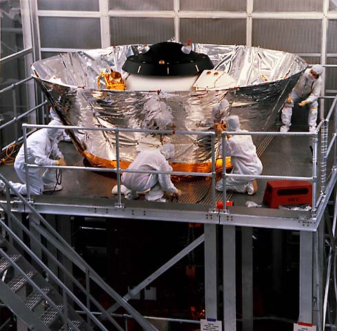
However, the SZ effect is interesting in its own right because it provides a way to understand how galaxy clusters have formed and evolved over the history of the Universe. Because the CMB comes to us from essentially the beginning of the Universe, it probes as far as can be probed by photons. What’s more, the SZ effect depends only on the angular size of the clusters and the temperature of their gas, it is not affected by the 1/r² dimming law that affects many astronomical measurements. Thus SZ provides a powerful means to study structures anywhere along the line of sight. One of the many telescopes studying the SZ effect is the South Pole Telescope. Animated Figure B.15.2 shows this telescope being built.

The South Pole Telescope (SPT) is one of several telescopes studying the SZ effect, which can be used to find galaxy clusters. Credit: SPT Collaboration.

In the next activity, you will examine several CMB maps to get a sense of the temperature and angular scales of variations in the CMB.

Understanding Cmb Anisotropy Maps

Figure A.15.1 presents maps of CMB anisotropy as observed by the COBE, WMAP, and Planck satellites. Use these maps to answer the questions below.

Figure A.15.1: Maps of the CMB, as observed by three different satellites. (Top) COBE. (Middle) WMAP. (Bottom) Planck. Credits: NASA/COBE Team, NASA/WMAP Science Team, ESA and the Planck Collaboration

A. Resolution and Angular Scale

1.

2.

3.

B. Temperature

1.

2.

C. Comparing With Known Objects.

1.

2.

3.

As with many astronomical measurements, CMB observations are often conducted from locations inhospitable to humans. The chosen locations tend to be high and dry in order to reduce the interference from Earth’s atmosphere. Though the CMB is everywhere, we go to these great lengths and exotic locations in order to get the most precise measurements. To date, there have been three satellites, over a dozen balloon-borne experiments, and more than three dozen ground-based experiments that have studied the CMB, with more to come in the future.

The advantage of satellite missions is that they can map the whole sky with high precision and without interference from the atmosphere. The disadvantages are that they often have a long development period and are costly. Experiments carried by long duration balloons around Antarctica fly at an altitude of about 120,000 feet (three to four times higher than a commercial airplane), above most of Earth’s atmosphere. A plethora of experiments have detected or constrained CMB anisotropy from the ground. The South Pole is an especially attractive site for CMB measurement because it has a stable atmosphere, has a high altitude (~10,000 feet), and is the driest place on Earth. Examples of other favorable locations include the California desert and the mountains of Chile.

Conducting CMB observations today is a team effort. It is often done in large collaborations where various group members make highly specialized contributions to the larger effort. Some team members build the telescopes or detectors, others make the observations, and still others are responsible for the data analysis in which the observations are compared with theoretical models. Figure 15.9a shows some of the telescopes and their instruments from recent CMB experiments and Figure 15.9b shows some CMB telescopes in action.

Figure 15.9a: A few of the many instruments used in recent CMB experiments: a close-up of the ACBAR feed horns and electronics, the BOOMERANG telescope , and the WMAP satellite. To date there have been more than 50 experiments designed to measure the CMB. Credits: Acbar Collaboration, NASA/COBE Team, BOOMERANG Collaboration

Figure 15.9b: Several recent CMB telescopes in action: the launch of the balloon-borne BOOMERANG telescope from the coast of Antarctica, DASI at sunset at the South Pole, the CBI dome in the mountains of Chile, and the launch of the WMAP satellite. Prime locations for microwave telescopes are high and dry, above as much of Earth’s atmosphere as possible. Credits: BOOMERANG Collaboration, DASI Collaboration, CBI Collaboration, NASA/WMAP Science Team

To help you visualize what the CMB would look like to you if you could see what some of these telescopes see, Figure 15.10 is a fanciful picture super-imposing a false-color map of the CMB on the launch site for the BOOMERANG balloon-borne telescope.

Figure 15.10: Fanciful image of what you might see in the sky if you could see what the BOOMERANG microwave telescope saw. The BOOMERANG map of the CMB is super-imposed to scale on the launch photo. Credit: BOOMERANG Collaboration.