
17.1: Evidence for Dark Energy


- Last updated
- Mar 3, 2023
- Save as PDF

( \newcommand{\kernel}{\mathrm{null}\,}\)
Login with LibreOne to view this question
NOTE: If you typically access ADAPT assignments through an LMS like Canvas, you should open this page there.
The Expansion Rate of the Universe Over Time
What does the expansion of the Universe look like as time passes? That is, if we could watch the Universe expand over its entire history, what would it look like? First we will look at the expansion rate today. We can do that using a Hubble diagram (Figure 17.1) for nearby galaxies. A Hubble diagram shows the velocities of galaxies plotted vs. their distances, as is discussed in Chapter 13.
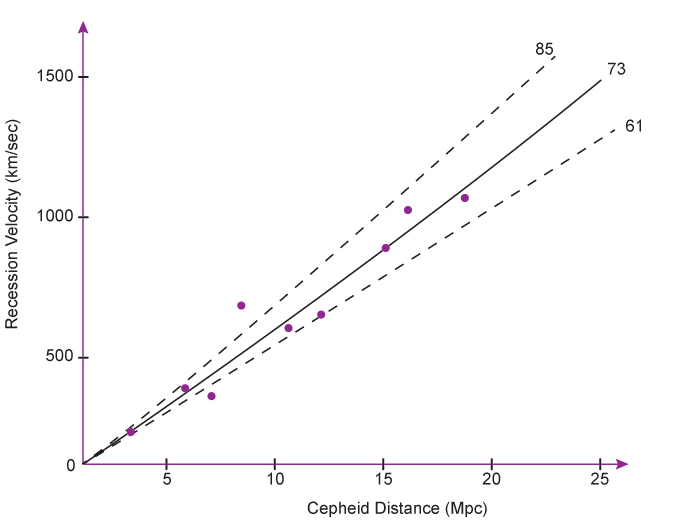
In this diagram, the expansion rate of the Universe is constant, as evidenced by the straight-line fit to the data. However, these galaxies are relatively nearby (so relatively close to us in lookback time as well). If we look at galaxies that are farther away in distance, we can measure the value of the Hubble parameter as we go farther back in time. Recall that the finite speed of light means greater distance means larger lookback time.
In the following activities, we will explore what a Hubble diagram looks like if the expansion rate is faster or slower or if it is increasing or decreasing. One thing to keep in mind is that the expansion history can be a little tricky to describe because of the early incident of Inflation. That event basically erased any earlier evidence of what the expansion might have been before. To avoid the ambiguity associated with the pre-inflation Universe, we will limit our inquiry to only the time after inflation occurred.
B. What if the expansion rate is faster or slower?
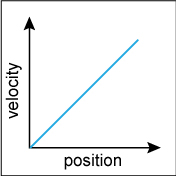
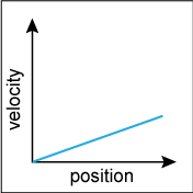
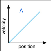
The slope of each graph in Figure A.17.1 is the Hubble parameter. On the left is a Hubble diagram with a slope of 70 km/s/Mpc. On the same scale are two other Hubble diagrams.

1.
Login with LibreOne to view this question
NOTE: If you typically access ADAPT assignments through an LMS like Canvas, you should open this page there.
2.
Login with LibreOne to view this question
NOTE: If you typically access ADAPT assignments through an LMS like Canvas, you should open this page there.
3.
Login with LibreOne to view this question
NOTE: If you typically access ADAPT assignments through an LMS like Canvas, you should open this page there.
4.
Login with LibreOne to view this question
NOTE: If you typically access ADAPT assignments through an LMS like Canvas, you should open this page there.
5.
Login with LibreOne to view this question
NOTE: If you typically access ADAPT assignments through an LMS like Canvas, you should open this page there.
6.
Login with LibreOne to view this question
NOTE: If you typically access ADAPT assignments through an LMS like Canvas, you should open this page there.
7.
Login with LibreOne to view this question
NOTE: If you typically access ADAPT assignments through an LMS like Canvas, you should open this page there.
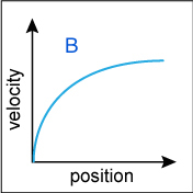
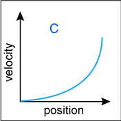
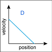
C. What if the Hubble parameter is not constant?
Figure A.17.2 shows four possible Hubble diagrams.
1.
Login with LibreOne to view this question
NOTE: If you typically access ADAPT assignments through an LMS like Canvas, you should open this page there.
2.
Login with LibreOne to view this question
NOTE: If you typically access ADAPT assignments through an LMS like Canvas, you should open this page there.
3.
Login with LibreOne to view this question
NOTE: If you typically access ADAPT assignments through an LMS like Canvas, you should open this page there.
4.
Login with LibreOne to view this question
NOTE: If you typically access ADAPT assignments through an LMS like Canvas, you should open this page there.
5.
Login with LibreOne to view this question
NOTE: If you typically access ADAPT assignments through an LMS like Canvas, you should open this page there.
6.
Login with LibreOne to view this question
NOTE: If you typically access ADAPT assignments through an LMS like Canvas, you should open this page there.
7.
Login with LibreOne to view this question
NOTE: If you typically access ADAPT assignments through an LMS like Canvas, you should open this page there.
8.
Login with LibreOne to view this question
NOTE: If you typically access ADAPT assignments through an LMS like Canvas, you should open this page there.
9.
Login with LibreOne to view this question
NOTE: If you typically access ADAPT assignments through an LMS like Canvas, you should open this page there.
10.
Login with LibreOne to view this question
NOTE: If you typically access ADAPT assignments through an LMS like Canvas, you should open this page there.
11.
Login with LibreOne to view this question
NOTE: If you typically access ADAPT assignments through an LMS like Canvas, you should open this page there.
12.
Login with LibreOne to view this question
NOTE: If you typically access ADAPT assignments through an LMS like Canvas, you should open this page there.
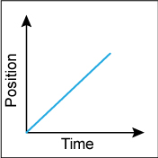
In the opening video for this chapter, we made an analogy between the expansion of the Universe and a ball in motion because in both cases we are dealing with the interplay of gravity and the energy of motion. In the next several activities, we will explore what these situations look like graphically.
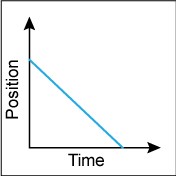
1. Imagine rolling a ball at constant speed away from you. What will its motion look like? (We assume that there is no friction in this example.) A graph of its position vs. time will resemble Figure A.17.3.
1.
Login with LibreOne to view this question
NOTE: If you typically access ADAPT assignments through an LMS like Canvas, you should open this page there.
2.
Login with LibreOne to view this question
NOTE: If you typically access ADAPT assignments through an LMS like Canvas, you should open this page there.
3.
Login with LibreOne to view this question
NOTE: If you typically access ADAPT assignments through an LMS like Canvas, you should open this page there.
4.
Login with LibreOne to view this question
NOTE: If you typically access ADAPT assignments through an LMS like Canvas, you should open this page there.
5.
Login with LibreOne to view this question
NOTE: If you typically access ADAPT assignments through an LMS like Canvas, you should open this page there.
6.
Login with LibreOne to view this question
NOTE: If you typically access ADAPT assignments through an LMS like Canvas, you should open this page there.
7.
Login with LibreOne to view this question
NOTE: If you typically access ADAPT assignments through an LMS like Canvas, you should open this page there.
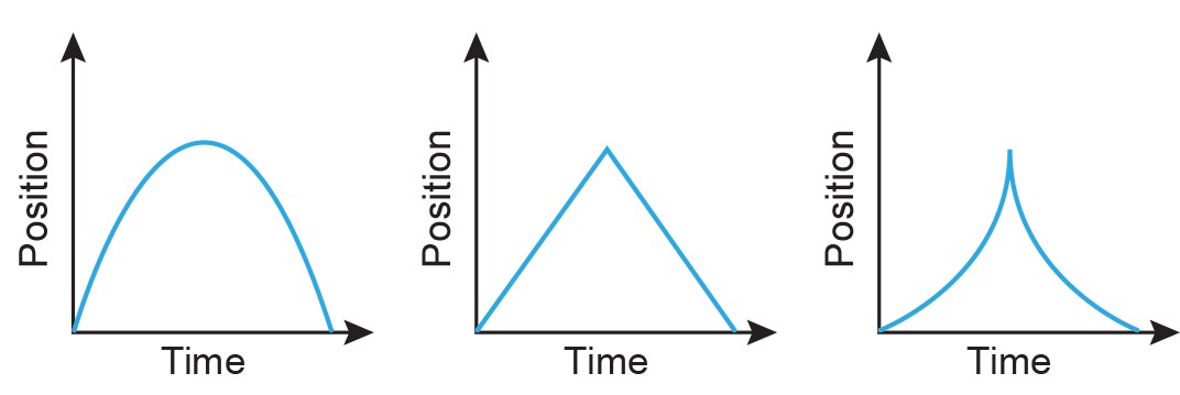
Imagine we throw a ball upward from Earth’s surface as in the last activity. At first the ball will be moving quickly upward. Under the influence of gravity the speed of the ball will slow over time, generally to the point of stopping. The ball will then reverse its motion and fall back to the surface with increasing speed.
This scenario is not the only one that we might see. It is possible to give the ball so much speed at the outset that it never slows enough to fall back to Earth. This speed is called escape velocity , and for an object launched from Earth’s surface it is about 11 km/s. But even if we throw the ball upward with escape velocity, or greater for that matter, it slows over time. It just does not slow fast enough for gravity to eventually halt its motion.
Given our intuitive understanding of gravity, we might expect that objects under an attractive gravitational influence will have their motion slowed if they initially are moving away from one another. Therefore, we might also conclude that the expansion of the Universe should have been slowing over time since all galaxies attract all other galaxies. But is this the correct scenario? In the following activity, we will examine how the scale factor of the Universe might change over time.
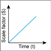
The scale factor of the Universe, S, describes how much the Universe has expanded (or contracted) over time, and a graph of S vs. time tells us how the rate of expansion has changed, if at all. If the expansion rate remains constant over time, a graph of S vs. t will look like the one in Figure A.17.6.
1.
Login with LibreOne to view this question
NOTE: If you typically access ADAPT assignments through an LMS like Canvas, you should open this page there.
You may have noticed that this diagram of scale factor vs. time resembles the Hubble diagrams in Figure 17.1 and Figure A.17.1, which show the position of galaxies on the x-axis and the velocity of galaxies on the y-axis. However, in the Hubble diagram, distant galaxies (and hence earlier times) are on the right, whereas here, earlier times are on the left. Both a scale factor vs. time and a Hubble diagram can be used to describe the expansion of the Universe.
In Figure A.17.7, we explore other possibilities for what the scale factor might do as time passes.
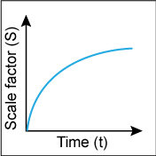
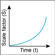

2. For which of the graphs does the scale factor (only) get bigger as time increases? (Check all that apply.)
Lef
Login with LibreOne to view this question
NOTE: If you typically access ADAPT assignments through an LMS like Canvas, you should open this page there.
3.
Login with LibreOne to view this question
NOTE: If you typically access ADAPT assignments through an LMS like Canvas, you should open this page there.
4.
Login with LibreOne to view this question
NOTE: If you typically access ADAPT assignments through an LMS like Canvas, you should open this page there.
5.
Login with LibreOne to view this question
NOTE: If you typically access ADAPT assignments through an LMS like Canvas, you should open this page there.
6.
Login with LibreOne to view this question
NOTE: If you typically access ADAPT assignments through an LMS like Canvas, you should open this page there.
7.
Login with LibreOne to view this question
NOTE: If you typically access ADAPT assignments through an LMS like Canvas, you should open this page there.
8.
Login with LibreOne to view this question
NOTE: If you typically access ADAPT assignments through an LMS like Canvas, you should open this page there.
We have seen two different ways to graphically represent the expansion of the Universe: a Hubble diagram (velocity vs. distance) and a diagram of scale factor vs. time. Place each of the following graphs in the correct bin, depending on whether it describes an expansion that is constant, slowing down, or speeding up.
Hint: Recall that when we are looking at far away galaxies, we are looking at earlier times in the history of the Universe.
The Expansion of the Universe is Accelerating
If we wish to measure the expansion of the Universe at large distances (early times), we must have a way to determine both the distance to objects and their recession speeds independently. The redshift is an easy way to determine a galaxy’s recession from us, but determining distances on large scales is more difficult. It requires a calibrated method that allows distance determinations independent of redshift—either a standard candle or a standard ruler is needed.
Type I supernovae turn out to be excellent standard candles; each can be calibrated and its luminosity determined to high precision. This particular kind of supernova occurs when a white dwarf star (of a particular composition) accretes enough material from a binary companion to become gravitationally unstable. The instability sets in when the white dwarf reaches 1.4 solar masses. Because the resulting explosions come from objects that are similar, with only slight variations, they all have nearly the same luminosity. This means that, once a measurement of their apparent brightness is made, their distance can be determined by comparing it to their intrinsic brightness.
Another property of Type I supernovae that suits them to studying the early expansion of the universe is their extreme brightness. They are so bright, in fact, that they can be seen to very great distances, and thus to very early times in the history of the Universe. This means that astronomers can use them to create a Hubble diagram that spans a large fraction of the past. So white dwarf supernovae are an ideal tool to show us whether the expansion rate of the Universe has been constant over time.
The quantities we actually observe for the supernovae are flux (or magnitude) and redshift. From these observations we must use some framework or model to interpret the meaning of our measurements. One model is the inverse-square behavior of light. Using this law, we can determine the distance (d) to a supernova from its measured flux (F) and the known luminosity (L).
F=L4πd2
Astronomers often work with the magnitude system instead of direct fluxes. Magnitudes are related to the logarithm of the flux. To learn more about magnitudes, see Going Further 3.6: The Magnitude System. The following activity explores how the brightness of a supernova (in magnitudes) depends on its distance.
Traditionally, the brightness of objects in optical light is expressed in terms of apparent magnitude (m) instead of flux (F). Correspondingly, the absolute magnitude (M) is used instead of luminosity (L). Like flux, the apparent magnitude relates to how bright an object appears to us. The absolute magnitude is a measure of its true brightness in absolute terms, like the luminosity. Specifically, M is the apparent magnitude an object would have if it were placed at a distance of 10 parsecs. As the distance increases the apparent brightness of an object will decrease, and so m will increase. (One counterintuitive aspect of the magnitude system is that fainter objects have larger values when measured in magnitudes.)
In terms of magnitudes, the inverse-square law becomes:
d=10(m−M+5)/5
From this expression, we can see that the distance depends on the quantity (m-M), the difference between the apparent magnitude and the absolute magnitude. This relationship can be expressed graphically:
Using the graph, answer the following questions.
1.
Login with LibreOne to view this question
NOTE: If you typically access ADAPT assignments through an LMS like Canvas, you should open this page there.
2.
Login with LibreOne to view this question
NOTE: If you typically access ADAPT assignments through an LMS like Canvas, you should open this page there.
3.
Login with LibreOne to view this question
NOTE: If you typically access ADAPT assignments through an LMS like Canvas, you should open this page there.
Another model we use is general relativity. In particular, we assume that Universe is homogeneous and isotropic. That assumption allows us to connect distance and redshift in a way that depends on cosmic parameters like the Hubble parameter and the amount and type of material in the Universe. The following activity will demonstrate how the content of the Universe affects the apparent brightness of objects as their redshift varies.
In this activity, you will vary the amount of matter in the Universe (matter fraction), along with the Hubble constant. In addition, you can change the amount of dark energy, a strange effect that causes the Universe to expand faster over time. We will look in more detail at what dark energy might be later in the chapter. You will notice that each of these quantities has an effect on the apparent brightness of a given object at a certain redshift (z). Again, the brightness is shown in terms of the difference in apparent magnitude (m) and absolute magnitude (M); larger (m–M) values mean fainter objects.
To create a graph, set the parameters to the values you want and choose “Graph Data.”
A. Effect of the Hubble constant
Set the parameters to the following and plot a graph:
- Hubble constant = 70
- Mass fraction = 1.0
- Redshift = 3
- Dark energy fraction = 0.0
1.
Login with LibreOne to view this question
NOTE: If you typically access ADAPT assignments through an LMS like Canvas, you should open this page there.
2.
Login with LibreOne to view this question
NOTE: If you typically access ADAPT assignments through an LMS like Canvas, you should open this page there.
3.
Login with LibreOne to view this question
NOTE: If you typically access ADAPT assignments through an LMS like Canvas, you should open this page there.
4.
Login with LibreOne to view this question
NOTE: If you typically access ADAPT assignments through an LMS like Canvas, you should open this page there.
Now set the Hubble constant to 140 while keeping the other parameters the same. Make a graph.
5.
Login with LibreOne to view this question
NOTE: If you typically access ADAPT assignments through an LMS like Canvas, you should open this page there.
B. Effect of the matter fraction
Clear the graph, set the parameters to the following, and plot a graph:
- Hubble constant = 70
- Mass fraction = 1.0
- Redshift = 3
- Dark energy fraction = 0.0
While keeping the other parameters the same, change the matter fraction to 0.5 and plot the graph. Also plot a matter fraction of 0.25.
1.
Login with LibreOne to view this question
NOTE: If you typically access ADAPT assignments through an LMS like Canvas, you should open this page there.
2.
Login with LibreOne to view this question
NOTE: If you typically access ADAPT assignments through an LMS like Canvas, you should open this page there.
C. Effect of dark energy
Clear the graph, set the parameters to the following, and plot a graph:
- Hubble constant = 70
- Mass fraction = 1.0
- Redshift = 3
- Dark energy fraction = 0.0
While keeping the other parameters the same, change the mass fraction to 0.5 and the dark energy fraction to 0.5 and plot the graph. Also make a graph with the mass fraction = 0.25 and the dark energy fraction = 0.75.
1.
Login with LibreOne to view this question
NOTE: If you typically access ADAPT assignments through an LMS like Canvas, you should open this page there.
2. I
Login with LibreOne to view this question
NOTE: If you typically access ADAPT assignments through an LMS like Canvas, you should open this page there.
In the previous activity, you saw how changing various cosmological parameters affected the expansion of the Universe. In particular, you should have seen that adding dark energy term to the energy content increased the magnitude of objects (i.e., decreased their apparent brightness) relative to a model that had no dark energy. This is because dark energy causes the expansion rate to speed up, which in turn changes the relationship between distance and velocity. The differences are quite small at low redshift but start to become apparent for objects at redshifts approaching or exceeding z ~ 1. Objects at such a high redshift are immensely far away. That means we must observe standard candles that have an extraordinarily large brightness, like supernovae, in order to see the effects of dark energy.
In the 1990s two groups of astronomers, the Supernova Cosmology Project and the High-Z Supernova Search, began to exploit Type I supernovae as standard candles. They worked independently and by the end of the decade both had enough supernovae in their sample to draw some conclusions about the expansion of the Universe. In an unexpected result, both groups found that the Universe is expanding faster over time, or in other words, that some sort of dark energy is present. Figure 17.2 combines the published results of both the teams. You can see that the supernovae, despite having quite a bit of scatter, favor the fainter (top) curve, the one including a dark energy fraction of 0.7 and matter fraction of 0.3. These results, from 1998 and 1999, were the first indication that the Universe contains dark energy. In fact, they suggest that the dark energy is the dominant component of the energy in the Universe, though its effects are currently only apparent on very large size scales.
.png?revision=1&size=bestfit&width=500)
For their initial discovery of dark energy, Saul Perlmutter of the Supernova Cosmology Project and Adam Riess and Brian Schmidt of the High-Z Supernova Search Team were jointly awarded the 2011 Nobel Prize in Physics. We will explore additional evidence for dark energy later in the chapter.