15.3: The equations of motion

First let us consider the motion of an asteroid under the gravitational influence of the Sun alone, ignoring perturbations from the other planets. We take the mass of the Sun to be M and the mass of the asteroid to be m. The force on the asteroid − and, of course, by Newton’s third law, the force on the Sun − is \( \frac{G M m}{r^{2}}\), where r is the distance between the two bodies. The two bodies are, of course, in motion around their common centre of mass, which, in the case of an asteroid, is very close to the centre of the Sun.

The acceleration of the asteroid towards the centre of mass is \(\frac{G M}{r^{2}}\), and the acceleration of the Sun towards the centre of mass is \(\frac{G m}{r^{2}}\). If we refer the motion to the Sun as origin, we see that the acceleration of the asteroid towards the Sun is \( \frac{G(M+m)}{r^{2}}\). In vector form we may write this as

\[\ddot{\mathbf{r}}=-\frac{G(M+m)}{r^{3}} \mathbf{r},\]

where r is a vector directed from the Sun towards the asteroid, with heliocentric rectangular components (x, y, z). These heliocentric coordinates could be either ecliptic coordinates, for which we have hitherto used the symbols (X, Y, Z); or they could be equatorial coordinates, for which we have hitherto used the symbols (ξ, η, ζ). The symbols (x, y, z) will be understood here to refer to either, at our convenience. It is more likely that we shall have available the equatorial rather than the ecliptic coordinates. The direction cosines of r are \( \left(\frac{x}{r}, \frac{y}{r}, \frac{z}{r}\right)\), and consequently the rectangular components of Equation 15.3.1 are

\[ \ddot{x}=-\frac{G(M+m)}{r^{3}} x\]

\[ \ddot{y} =-\frac{G(M+m)}{r^{3}} y\]

\[\ddot{z} =-\frac{G(M+m)}{r^{3}} z\]

These are the Equations of motion of the asteroid with respect to the Sun as origin. The quantities \(x, y, z, r\left(=\sqrt{x^{2}+y^{2}+z^{2}}\right)\) are, of course, functions of time. The solution of these Equations describe the elliptical (or other conic section) orbits of the asteroid and all the other properties that we have discussed in previous chapters.

If we are using ecliptic coordinates (X, Y, Z), the X-axis is directed towards the First Point of Aries, the Y-axis is directed along the direction of increasing ecliptic longitude, and the Z-axis is directed towards the north pole of the ecliptic.

If we are using equatorial coordinates (ξ, η, ζ), the ξ-axis is directed towards the First Point of Aries, the η-axis is directed along the direction of 6 hours right ascension, and the ζ-axis is directed towards the north celestial pole. The Earth will be on the X- or ξaxis in September (not March).

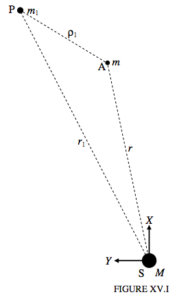
Now let us introduce a third body, a perturbing planet, such as, perhaps, Jupiter. We’ll suppose that its mass is m₁, that its distance from the Sun is r₁ and its distance from the asteroid is ρ₁ (see figure XV.I, in which S is the Sun, A is the asteroid, and P is the perturbing planet). This is now a three-body problem and a general solution in terms of algebraic functions is not possible, and it has to be solved by numerical computation.

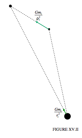
In addition to the accelerations of the asteroid towards the Sun and the Sun towards the asteroid described on page 3, used in developing Equations 15.3.1-4, we now have also to consider the accelerations of the asteroid and the Sun towards the perturbing planet, as indicated in figure XV.II.

The x-components of these are \( \frac{G m_{1}}{\rho_{1}^{2}} \times \frac{x_{1}-x}{\rho_{1}}\) and \( \frac{G m_{1}}{r_{1}^{2}} \times \frac{x_{1}}{r_{1}}\), and so the additional acceleration of A, relative to the Sun, in the X-direction is \( G m_{1}\left(\frac{x_{1}-x}{\rho_{1}^{3}}-\frac{x_{1}}{r_{1}^{3}}\right)\), and this has now to be added to the right hand side of Equation 15.3.2:

\[ \ddot{x}=-\frac{G(M+m)}{r^{3}} x+G m_{1}\left(\frac{x_{1}-x}{\rho_{1}^{3}}-\frac{x_{1}}{r_{1}^{3}}\right)\]

Neither G nor M are known to great precision, but the product GM is known to very great precision. Indeed in computational practice we make use of the Gaussian constant \( k=\sqrt{\frac{G M}{a_{0}}}\), where a₀ is the astronomical unit of length. This constant has dimension T⁻¹ and is equal to the angular velocity of a particle of negligible mass in circular orbit of radius 1 au around the Sun, which is 0.017 202 098 95 radians per mean solar day. Therefore in computational practice, Equation 15.3.5 is generally written as

\[ \ddot{x}=-\frac{k^{2}(1+m)}{r^{3}} x+k^{2} m_{1}\left(\frac{x_{1}-x}{\rho_{1}^{3}}-\frac{x_{1}}{r_{1}^{3}}\right),\]

in which the units of mass, length and time are, respectively, solar mass, astronomical unit, and mean solar day. Recall that m is the mass of the asteroid whose orbit we are computing, and m₁ is the mass of the perturbing planet, and that the origin of coordinates is the centre of the Sun. Similar Equations apply to the y- and z-components:

\[ \ddot{y}=-\frac{k^{2}(1+m)}{r^{3}} y+k^{2} m_{1}\left(\frac{y_{1}-y}{\rho_{1}^{3}}-\frac{y_{1}}{r_{1}^{3}}\right)\]

\[\ddot{z}=-\frac{k^{2}(1+m)}{r^{3}} z+k^{2} m_{1}\left(\frac{z_{1}-z}{\rho_{1}^{3}}-\frac{z_{1}}{r_{1}^{3}}\right)\]

If we add the perturbations from all the major planets from Mercury (M) to Neptune (N), these Equations become, of course,

\[ \ddot{x}=-\frac{k^{2}(1+m)}{r^{3}} x+k^{2} \sum_{i=M}^{N} m_{i}\left(\frac{x_{i}-x}{\rho_{i}^{3}}-\frac{x_{i}}{r_{i}^{3}}\right)\]

and similar Equations in y and z.

In the case of an asteroid or a comet, it may be permissible to neglect m in this Equation (i.e. set m = 0), but not, of course, m₁. We shall do that here, so the Equation of motion in x becomes

\[\ddot{x}=-k^{2} \frac{x}{r^{3}}+k^{2} \sum_{i=\mathrm{M}}^{\mathrm{N}} m_{i}\left(\frac{x_{i}-x}{\rho_{i}^{3}}-\frac{x_{i}}{r_{i}^{3}}\right),\]

with similar Equations in y and z.

The x, x_i, ρ_i, r_i, etc., are numerical data, which have to be supplied by independent computations (subroutines) for all the planets. As stated at the end of the previous Section, we suppose that we have subroutines in our program that we can call upon to calculate these data at any date. We also pointed out that the Equations of motion are valid for either ecliptic or equatorial coordinates, although the coordinates of the planets are more likely to be available is equatorial rather than ecliptic coordinates. They are all functions of time, so that, in effect, we have to develop numerical methods for integrating Equations of the form, where f(t) is not an algebraic expression, but rather a table of numerical values.

\[\ddot{x}=f(t)\]

That is to say

\[\frac{d \dot{x}}{d t}=f(t).\]

We suppose that we know x& at the epoch of osculation. Then we can find \(\dot{x}\) at any subsequent date by any standard technique of numerical integration, such as Simpson’s or Weddle’s Rules, or Gaussian quadrature, or by a Runge-Kutta process. Thus we now have a table of \(\dot{x}\) as a function of time:

\[\dot{x}=g(t)\]

That is to say

\[\frac{d x}{d t}=g(t)\]

We integrate a second time, until we arrive at both x and \(\dot{x}\) at some subsequent epoch of osculation (perhaps 200, or 40, days into the future). Repeat with the y and z components, so we eventually have a new set of \((x, y, z, \dot{x}, \dot{y}, \dot{z})\) for a later epoch, and hence also of a, e, i, Ω, ω, T.