23.3: Energy and the Simple Harmonic Oscillator

Let’s consider the block-spring system of Example 23.2 in which the block is initially stretched an amount \(x_{0}>0\) from the equilibrium position and is released from rest, \(v_{x, 0}=0\). We shall consider three states: state 1, the initial state; state 2, at an arbitrary time in which the position and velocity are non-zero; and state 3, when the object first comes back to the equilibrium position. We shall show that the mechanical energy has the same value for each of these states and is constant throughout the motion. Choose the equilibrium position for the zero point of the potential energy.

State 1: all the energy is stored in the object-spring potential energy, \(U_{1}=(1 / 2) k x_{0}^{2}\). The object is released from rest so the kinetic energy is zero, \(K_{1}=0\) The total mechanical energy is then

\[E_{1}=U_{1}=\frac{1}{2} k x_{0}^{2} \nonumber \]

State 2: at some time t , the position and x -component of the velocity of the object are given by

\[\begin{aligned}
x(t) &=x_{0} \cos (\sqrt{\frac{k}{m}} t) \\
v_{x}(t) &=-\sqrt{\frac{k}{m} x_{0} \sin (\sqrt{\frac{k}{m}} t})
\end{aligned} \nonumber \]

The kinetic energy is

\[K_{2}=\frac{1}{2} m v^{2}=\frac{1}{2} k x_{0}^{2} \sin ^{2}(\sqrt{\frac{k}{m}} t) \nonumber \]

and the potential energy is

\[U_{2}=\frac{1}{2} k x^{2}=\frac{1}{2} k x_{0}^{2} \cos ^{2}(\sqrt{\frac{k}{m}} t) \nonumber \]

The mechanical energy is the sum of the kinetic and potential energies

\[\begin{array}{l}
E_{2}=K_{2}+U_{2}=\frac{1}{2} m v_{x}^{2}+\frac{1}{2} k x^{2} \\
=\frac{1}{2} k x_{0}^{2}\left(\cos ^{2}(\sqrt{\frac{k}{m}} t)+\sin ^{2}(\sqrt{\frac{k}{m}} t)\right) \\
=\frac{1}{2} k x_{0}^{2}
\end{array} \nonumber \]

where we used the identity that \(\cos ^{2} \omega_{0} t+\sin ^{2} \omega_{0} t=1\) and that \(\omega_{0}=\sqrt{k / m}\) (Equation (23.2.6)).

The mechanical energy in state 2 is equal to the initial potential energy in state 1, so the mechanical energy is constant. This should come as no surprise; we isolated the object spring system so that there is no external work performed on the system and no internal non-conservative forces doing work.

Figure 23.5 State 3 at equilibrium and in motion

State 3: now the object is at the equilibrium position so the potential energy is zero, U3 = 0 , and the mechanical energy is in the form of kinetic energy (Figure 23.5).

\[E_{3}=K_{3}=\frac{1}{2} m v_{\mathrm{eq}}^{2} \nonumber \]

Because the system is closed, mechanical energy is constant,

\[E_{1}=E_{3} \nonumber \]

Therefore the initial stored potential energy is released as kinetic energy,

\[\frac{1}{2} k x_{0}^{2}=\frac{1}{2} m v_{\mathrm{eq}}^{2} \nonumber \]

and the x -component of velocity at the equilibrium position is given by

\[v_{\mathrm{x}, \mathrm{eq}}=\pm \sqrt{\frac{k}{m}} x_{0} \nonumber \]

Note that the plus-minus sign indicates that when the block is at equilibrium, there are two possible motions: in the positive x -direction or the negative x -direction. If we take \(x_{0}>0\), then the block starts moving towards the origin, and \(\mathcal{V}_{\mathrm{x}, \mathrm{eq}}\) will be negative the first time the block moves through the equilibrium position.

We can show more generally that the mechanical energy is constant at all times as follows. The mechanical energy at an arbitrary time is given by

\[E=K+U=\frac{1}{2} m v_{x}^{2}+\frac{1}{2} k x^{2} \nonumber \]

Differentiate Equation (23.3.10)

\[\frac{d E}{d t}=m v_{x} \frac{d v_{x}}{d t}+k x \frac{d x}{d t}=v_{x}\left(m \frac{d^{2} x}{d t^{2}}+k x\right) \nonumber \]

Now substitute the simple harmonic oscillator equation of motion, (Equation (23.2.1) ) into Equation (23.3.11) yielding

\[\frac{d E}{d t}=0 \nonumber \]

demonstrating that the mechanical energy is a constant of the motion.

Simple Pendulum: Force Approach

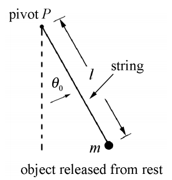
A pendulum consists of an object hanging from the end of a string or rigid rod pivoted about the point P . The object is pulled to one side and allowed to oscillate. If the object has negligible size and the string or rod is massless, then the pendulum is called a simple pendulum. Consider a simple pendulum consisting of a massless string of length l and a point-like object of mass m attached to one end, called the bob. Suppose the string is fixed at the other end and is initially pulled out at an angle \(\theta_{0}\) from the vertical and released from rest (Figure 23.6). Neglect any dissipation due to air resistance or frictional forces acting at the pivot.

Figure 23.6 Simple pendulum

Let’s choose polar coordinates for the pendulum as shown in Figure 23.7a along with the free-body force diagram for the suspended object (Figure 23.7b). The angle \(\theta\) is defined with respect to the equilibrium position. When \(\theta>0\), the bob is has moved to the right, and when \(\theta<0\), the bob has moved to the left. The object will move in a circular arc centered at the pivot point. The forces on the object are the tension in the string \(\overrightarrow{\mathbf{T}}=-T \hat{\mathbf{r}}\) and gravity \(m \overrightarrow{\mathbf{g}}\). The gravitation force on the object has \(\hat{\mathbf{r}}\)- and \(\hat{\theta}\)- component given by

\[m \overrightarrow{\mathbf{g}}=m g(\cos \theta \hat{\mathbf{r}}-\sin \theta \hat{\boldsymbol{\theta}}) \nonumber \]

Figure 23.7 (b) free-body force diagram

Our concern is with the tangential component of the gravitational force,

\[F_{\theta}=-m g \sin \theta \nonumber \]

The sign in Equation (23.3.14) is crucial; the tangential force tends to restore the pendulum to the equilibrium value \(\theta=0\). If \(\theta>0, F_{\theta}<0\) and if \(\theta<0, F_{\theta}>0\) where we are that because the string is flexible, the angle θ is restricted to the range \(-\pi / 2<\theta<\pi / 2\). (For angles \(|\theta|>\pi / 2\) the string would go slack.) In both instances the tangential component of the force is directed towards the equilibrium position. The tangential component of acceleration is

\[a_{\theta}=l \alpha=l \frac{d^{2} \theta}{d t^{2}} \nonumber \]

Newton’s Second Law, \(F_{\theta}=m a_{\theta}\), yields

\[-m g l \sin \theta=m l^{2} \frac{d^{2} \theta}{d t^{2}} \nonumber \]

We can rewrite this equation is the form

\[\frac{d^{2} \theta}{d t^{2}}=-\frac{g}{l} \sin \theta \nonumber \]

This is not the simple harmonic oscillator equation although it still describes periodic motion. In the limit of small oscillations, \(\sin \theta \cong \theta\), Equation (23.3.17) becomes

\[\frac{d^{2} \theta}{d t^{2}} \cong-\frac{g}{l} \theta \nonumber \]

This equation is similar to the object-spring simple harmonic oscillator differential equation

\[\frac{d^{2} x}{d t^{2}}=-\frac{k}{m} x \nonumber \]

By comparison with Equation (23.2.6) the angular frequency of oscillation for the pendulum is approximately

\[\omega_{0} \simeq \sqrt{\frac{g}{l}} \nonumber \]

with period

\[T=\frac{2 \pi}{\omega_{0}} \simeq 2 \pi \sqrt{\frac{l}{g}} \nonumber \]

The solutions to Equation (23.3.18) can be modeled after Equation (23.2.21). With the initial conditions that the pendulum is released from rest, \(\frac{d \theta}{d t}(t=0)=0\), at a small angle \(\theta(t=0)=\theta_{0}\), the angle the string makes with the vertical as a function of time is given by

\[\theta(t)=\theta_{0} \cos \left(\omega_{0} t\right)=\theta_{0} \cos \left(\frac{2 \pi}{T} t\right)=\theta_{0} \cos (\sqrt{\frac{g}{l}} t) \nonumber \]

The z -component of the angular velocity of the bob is

\[\omega_{z}(t)=\frac{d \theta}{d t}(t)=-\sqrt{\frac{g}{l}} \theta_{0} \sin (\sqrt{\frac{g}{l}} t) \nonumber \]

Keep in mind that the component of the angular velocity \(\omega_{z}=d \theta / d t\) changes with time in an oscillatory manner (sinusoidally in the limit of small oscillations). The angular frequency \(\omega_{0}\) is a parameter that describes the system. The z -component of the angular velocity \(\omega_{z}(t)\) besides being time-dependent, depends on the amplitude of oscillation \(\theta_{0}\). In the limit of small oscillations, \(\omega_{0}\) does not depend on the amplitude of oscillation.

The fact that the period is independent of the mass of the object follows algebraically from the fact that the mass appears on both sides of Newton’s Second Law and hence cancels. Consider also the argument that is attributed to Galileo: if a pendulum, consisting of two identical masses joined together, were set to oscillate, the two halves would not exert forces on each other. So, if the pendulum were split into two pieces, the pieces would oscillate the same as if they were one piece. This argument can be extended to simple pendula of arbitrary masses.

Simple Pendulum: Energy Approach

We can use energy methods to find the differential equation describing the time evolution of the angle \(\theta\). When the string is at an angle \(\theta\) with respect to the vertical, the gravitational potential energy (relative to a choice of zero potential energy at the bottom of the swing where \(\theta=0\) as shown in Figure 23.8) is given by

\[U=m g l(1-\cos \theta) \nonumber \]

The θ -component of the velocity of the object is given by \(v_{\theta}=l(d \theta / d t)\) so the kinetic energy is

\[K=\frac{1}{2} m v^{2}=\frac{1}{2} m\left(l \frac{d \theta}{d t}\right)^{2} \nonumber \]

Figure 23.8 Energy diagram for simple pendulum

The mechanical energy of the system is then

\[E=K+U=\frac{1}{2} m\left(l \frac{d \theta}{d t}\right)^{2}+m g l(1-\cos \theta) \nonumber \]

Because we assumed that there is no non-conservative work (i.e. no air resistance or frictional forces acting at the pivot), the energy is constant, hence

\[\begin{array}{l}
0=\frac{d E}{d t}=\frac{1}{2} m 2 l^{2} \frac{d \theta}{d t} \frac{d^{2} \theta}{d t^{2}}+m g l \sin \theta \frac{d \theta}{d t} \\
=m l^{2} \frac{d \theta}{d t}\left(\frac{d^{2} \theta}{d t^{2}}+\frac{g}{l} \sin \theta\right)
\end{array} \nonumber \]

There are two solutions to this equation; the first one \(d \theta / d t=0\) is the equilibrium solution. That the z -component of the angular velocity is zero means the suspended object is not moving. The second solution is the one we are interested in

\[\frac{d^{2} \theta}{d t^{2}}+\frac{g}{l} \sin \theta=0 \nonumber \]

which is the same differential equation (Equation (23.3.16)) that we found using the force method.

We can find the time \(t_{1}\) that the object first reaches the bottom of the circular arc by setting \(\theta\left(t_{1}\right)=0\) in Equation (23.3.22)

\[0=\theta_{0} \cos \left(\sqrt{\frac{g}{l}} t_{1}\right) \nonumber \]

This zero occurs when the argument of the cosine satisfies

\[\sqrt{\frac{g}{l}} t_{1}=\frac{\pi}{2} \nonumber \]

The z -component of the angular velocity at time \(t_{1}\) is therefore

\[\frac{d \theta}{d t}\left(t_{1}\right)=-\sqrt{\frac{g}{l}} \theta_{0} \sin \left(\sqrt{\frac{g}{l}} t_{1}\right)=-\sqrt{\frac{g}{l}} \theta_{0} \sin \left(\frac{\pi}{2}\right)=-\sqrt{\frac{g}{l}} \theta_{0} \nonumber \]

Note that the negative sign means that the bob is moving in the negative \(\hat{\boldsymbol{\theta}}\)-direction when it first reaches the bottom of the arc. The θ-component of the velocity at time \(t_{1}\) is therefore

\[v_{\theta}\left(t_{1}\right) \equiv v_{1}=l \frac{d \theta}{d t}\left(t_{1}\right)=-l \sqrt{\frac{g}{l}} \theta_{0} \sin \left(\sqrt{\frac{g}{l}} t_{1}\right)=-\sqrt{l g} \theta_{0} \sin \left(\frac{\pi}{2}\right)=-\sqrt{\lg } \theta_{0} \cdot(23.3 .32) \nonumber \]

We can also find the components of both the velocity and angular velocity using energy methods. When we release the bob from rest, the energy is only potential energy

\[E=U_{0}=m g l\left(1-\cos \theta_{0}\right) \cong m g l \frac{\theta_{0}^{2}}{2} \nonumber \]

where we used the approximation that \(\cos \theta_{0} \cong 1-\theta_{0}^{2} / 2\). When the bob is at the bottom of the arc, the only contribution to the mechanical energy is the kinetic energy given by

\[K_{1}=\frac{1}{2} m v_{1}^{2} \nonumber \]

Because the energy is constant, we have that \(U_{0}=K_{1}\) or

\[m g l \frac{\theta_{0}^{2}}{2}=\frac{1}{2} m v_{1}^{2} \nonumber \]

We can solve for the θ -component of the velocity at the bottom of the arc

\[v_{\theta, 1}=\pm \sqrt{g l} \theta_{0} \nonumber \]

The two possible solutions correspond to the different directions that the motion of the bob can have when at the bottom. The z -component of the angular velocity is then

\[\frac{d \theta}{d t}\left(t_{1}\right)=\frac{v_{1}}{l}=\pm \sqrt{\frac{g}{l}} \theta_{0} \nonumber \]

in agreement with our previous calculation.

If we do not make the small angle approximation, we can still use energy techniques to find the θ-component of the velocity at the bottom of the arc by equating the energies at the two positions

\[m g l\left(1-\cos \theta_{0}\right)=\frac{1}{2} m v_{1}^{2} \nonumber \]

\[v_{\theta, 1}=\pm \sqrt{2 g l\left(1-\cos \theta_{0}\right)} \nonumber \]

Simple Pendulum: Energy Approach

We can use energy methods to find the differential equation describing the time evolution of the angle \(\theta\). When the string is at an angle \(\theta\) with respect to the vertical, the gravitational potential energy (relative to a choice of zero potential energy at the bottom of the swing where \(\theta=0\) as shown in Figure 23.8) is given by

\[U=m g l(1-\cos \theta) \nonumber \]

The θ -component of the velocity of the object is given by \(v_{\theta}=l(d \theta / d t)\) so the kinetic energy is

\[K=\frac{1}{2} m v^{2}=\frac{1}{2} m\left(l \frac{d \theta}{d t}\right)^{2} \nonumber \]

Figure 23.8 Energy diagram for simple pendulum

The mechanical energy of the system is then

\[E=K+U=\frac{1}{2} m\left(l \frac{d \theta}{d t}\right)^{2}+m g l(1-\cos \theta) \nonumber \]

Because we assumed that there is no non-conservative work (i.e. no air resistance or frictional forces acting at the pivot), the energy is constant, hence

\[\begin{array}{l}
0=\frac{d E}{d t}=\frac{1}{2} m 2 l^{2} \frac{d \theta}{d t} \frac{d^{2} \theta}{d t^{2}}+m g l \sin \theta \frac{d \theta}{d t} \\
=m l^{2} \frac{d \theta}{d t}\left(\frac{d^{2} \theta}{d t^{2}}+\frac{g}{l} \sin \theta\right)
\end{array} \nonumber \]

There are two solutions to this equation; the first one \(d \theta / d t=0\) is the equilibrium solution. That the z -component of the angular velocity is zero means the suspended object is not moving. The second solution is the one we are interested in

\[\frac{d^{2} \theta}{d t^{2}}+\frac{g}{l} \sin \theta=0 \nonumber \]

which is the same differential equation (Equation (23.3.16)) that we found using the force method.

We can find the time \(t_{1}\) that the object first reaches the bottom of the circular arc by setting \(\theta\left(t_{1}\right)=0\) in Equation (23.3.22)

\[0=\theta_{0} \cos \left(\sqrt{\frac{g}{l}} t_{1}\right) \nonumber \]

This zero occurs when the argument of the cosine satisfies

\[\sqrt{\frac{g}{l}} t_{1}=\frac{\pi}{2} \nonumber \]

The z -component of the angular velocity at time \(t_{1}\) is therefore

\[\frac{d \theta}{d t}\left(t_{1}\right)=-\sqrt{\frac{g}{l}} \theta_{0} \sin \left(\sqrt{\frac{g}{l}} t_{1}\right)=-\sqrt{\frac{g}{l}} \theta_{0} \sin \left(\frac{\pi}{2}\right)=-\sqrt{\frac{g}{l}} \theta_{0} \nonumber \]

Note that the negative sign means that the bob is moving in the negative \(\hat{\boldsymbol{\theta}}\)-direction when it first reaches the bottom of the arc. The θ-component of the velocity at time \(t_{1}\) is therefore

\[v_{\theta}\left(t_{1}\right) \equiv v_{1}=l \frac{d \theta}{d t}\left(t_{1}\right)=-l \sqrt{\frac{g}{l}} \theta_{0} \sin \left(\sqrt{\frac{g}{l}} t_{1}\right)=-\sqrt{l g} \theta_{0} \sin \left(\frac{\pi}{2}\right)=-\sqrt{\lg } \theta_{0} \cdot(23.3 .32) \nonumber \]

We can also find the components of both the velocity and angular velocity using energy methods. When we release the bob from rest, the energy is only potential energy

\[E=U_{0}=m g l\left(1-\cos \theta_{0}\right) \cong m g l \frac{\theta_{0}^{2}}{2} \nonumber \]

where we used the approximation that \(\cos \theta_{0} \cong 1-\theta_{0}^{2} / 2\). When the bob is at the bottom of the arc, the only contribution to the mechanical energy is the kinetic energy given by

\[K_{1}=\frac{1}{2} m v_{1}^{2} \nonumber \]

Because the energy is constant, we have that \(U_{0}=K_{1}\) or

\[m g l \frac{\theta_{0}^{2}}{2}=\frac{1}{2} m v_{1}^{2} \nonumber \]

We can solve for the θ -component of the velocity at the bottom of the arc

\[v_{\theta, 1}=\pm \sqrt{g l} \theta_{0} \nonumber \]

The two possible solutions correspond to the different directions that the motion of the bob can have when at the bottom. The z -component of the angular velocity is then

\[\frac{d \theta}{d t}\left(t_{1}\right)=\frac{v_{1}}{l}=\pm \sqrt{\frac{g}{l}} \theta_{0} \nonumber \]

in agreement with our previous calculation.

If we do not make the small angle approximation, we can still use energy techniques to find the θ-component of the velocity at the bottom of the arc by equating the energies at the two positions

\[m g l\left(1-\cos \theta_{0}\right)=\frac{1}{2} m v_{1}^{2} \nonumber \]

\[v_{\theta, 1}=\pm \sqrt{2 g l\left(1-\cos \theta_{0}\right)} \nonumber \]