
23.2: Simple Harmonic Motion- Analytic

( \newcommand{\kernel}{\mathrm{null}\,}\)
Our first example of a system that demonstrates simple harmonic motion is a springobject system on a frictionless surface, shown in Figure 23.2
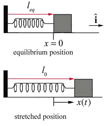
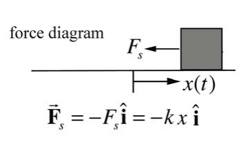
The object is attached to one end of a spring. The other end of the spring is attached to a wall at the left in Figure 23.2. Assume that the object undergoes one-dimensional motion. The spring has a spring constant k and equilibrium length leq Choose the origin at the equilibrium position and choose the positive x -direction to the right in the Figure 23.2. In the figure, x>0 corresponds to an extended spring, and x<0 to a compressed spring. Define x(t) to be the position of the object with respect to the equilibrium position. The force acting on the spring is a linear restoring force, Fx=−kx (Figure 23.3). The initial conditions are as follows. The spring is initially stretched a distance l0 and given some initial speed v0 to the right away from the equilibrium position. The initial position of the stretched spring from the equilibrium position (our choice of origin) is x0=(l0−leq)>0 and its initial x -component of the velocity is vx,0=v0>0.
Newton’s Second law in the x -direction becomes
−kx=md2xdt2
This equation of motion, Equation (23.2.1), is called the simple harmonic oscillator equation (SHO). Because the spring force depends on the distance x , the acceleration is not constant. Equation (23.2.1) is a second order linear differential equation, in which the second derivative of the dependent variable is proportional to the negative of the dependent variable,
d2xdt2=−kmx
In this case, the constant of proportionality is k/m.
Equation (23.2.2) can be solved from energy considerations or other advanced techniques but instead we shall first guess the solution and then verify that the guess satisfies the SHO differential equation (see Appendix 22.3.A for a derivation of the solution).
We are looking for a position function x(t) such that the second time derivative position function is proportional to the negative of the position function. Since the sine and cosine functions both satisfy this property, we make a preliminary ansatz (educated guess) that our position function is given by
x(t)=Acos((2π/T)t)=Acos(ω0t)
where ω0 is the angular frequency (as of yet, undetermined).
We shall now find the condition that the angular frequency ω0 must satisfy in order to insure that the function in Equation (23.2.3) solves the simple harmonic oscillator equation, Equation (23.2.1). The first and second derivatives of the position function are given by
dxdt=−ω0Asin(ω0t)d2xdt2=−ω20Acos(ω0t)=−ω20x
Substitute the second derivative, the second expression in Equation (23.2.4), and the position function, Equation (23.2.3), into the SHO Equation (23.2.1), yielding
−ω20Acos(ω0t)=−kmAcos(ω0t)
Equation (23.2.5) is valid for all times provided that
ω0=√km
The period of oscillation is then
T=2πω0=2π√mk
One possible solution for the position of the block is
x(t)=Acos(√kmt)
and therefore by differentiation, the x -component of the velocity of the block is
vx(t)=−√kmAsin(√kmt)
Note that at t=0, the position of the object is x0≡x(t=0)=A since cos(0)=1 and the velocity is vx,0≡vx(t=0)=0 since sin(0)=0. The solution in (23.2.8) describes an object that is released from rest at an initial position A=x0, but does not satisfy the initial velocity condition, vx(t=0)=vx,0≠0. We can try a sine function as another possible solution,
x(t)=Bsin(√kmt)
This function also satisfies the simple harmonic oscillator equation because
d2xdt2=−kmBsin(√kmt)=−ω20x
where ω0=√k/m. The x -component of the velocity associated with Equation (23.2.10) is
vx(t)=dxdt=√kmBcos(√kmt)
The proposed solution in Equation (23.2.10) has initial conditions x0≡x(t=0)=0 and vx,0≡vx(t=0)=(√k/m)B, thus B=vx,0/√k/m This solution describes an object that is initially at the equilibrium position but has an initial non-zero x -component of the velocity, vx,0≠0
General Solution of Simple Harmonic Oscillator Equation
Suppose x1(t) and x2(t) are both solutions of the simple harmonic oscillator equation,
d2dt2x1(t)=−kmx1(t)d2dt2x2(t)=−kmx2(t)
Then the sum x(t)=x1(t)+x2(t) of the two solutions is also a solution. To see this, consider
d2x(t)dt2=d2dt2(x1(t)+x2(t))=d2x1(t)dt2+d2x2(t)dt2
Using the fact that x1(t) and x2(t) both solve the simple harmonic oscillator equation (23.2.13), we see that
d2dt2x(t)=−kmx1(t)+−kmx2(t)=−km(x1(t)+x2(t))=−kmx(t)
Thus the linear combination x(t)=x1(t)+x2(t) is also a solution of the SHO equation, Equation (23.2.1). Therefore the sum of the sine and cosine solutions is the general solution,
x(t)=Ccos(ω0t)+Dsin(ω0t)
where the constant coefficients C and D depend on a given set of initial conditions x0≡x(t=0) and vx,0≡vx(t=0) where x0 and vx,0 are constants. For this general solution, the x -component of the velocity of the object at time t is then obtained by differentiating the position function,
vx(t)=dxdt=−ω0Csin(ω0t)+ω0Dcos(ω0t)
To find the constants C and D , substitute t = 0 into the Equations (23.2.16) and (23.2.17). Because cos(0)=1 and sin(0)=0, the initial position at time t = 0 is
x0≡x(t=0)=C
The x -component of the velocity at time t = 0 is
vx,0=vx(t=0)=−ω0Csin(0)+ω0Dcos(0)=ω0D
Thus
C=x0 and D=vx,0ω0
and the x -component of the velocity of the object-spring system is
vx(t)=−√kmx0sin(√kmt)+vx,0cos(√kmt)
Although we had previously specified x0>0 and vx,0>0, Equation (23.2.21) is seen to be a valid solution of the SHO equation for any values of x0 and vx,0.
Example 23.1: Phase and Amplitude
Show that x(t)=Ccosω0t+Dsinω0t=Acos(ω0t+ϕ), where A=(C2+D2)1/2>0 and ϕ=tan−1(−D/C)
Solution: Use the identity Acos(ω0t+ϕ)=Acos(ω0t)cos(ϕ)−Asin(ω0t)sin(ϕ). Thus Ccos(ω0t)+Dsin(ω0t)=Acos(ω0t)cos(ϕ)−Asin(ω0t)sin(ϕ) Comparing coefficients we see that C=Acosϕ and D=−Asinϕ. Therefore
(C2+D2)1/2=A2(cos2ϕ+sin2ϕ)=A2
We choose the positive square root to ensure that A>0, and thus
A=(C2+D2)1/2tanϕ=sinϕcosϕ=−D/AC/A=−DC
ϕ=tan−1(−D/C)
Thus the position as a function of time can be written as
x(t)=Acos(ω0t+ϕ)
In Equation (23.2.25) the quantity ω0t+ϕ is called the phase, and ϕ is called the phase constant. Because cos(ω0t+ϕ) varies between +1 and −1 , and A>0 A is the amplitude defined earlier. We now substitute Equation (23.2.20) into Equation (23.2.23) and find that the amplitude of the motion described in Equation (23.2.21), that is, the maximum value of x(t), and the phase are given by
A=√x20+(vx,0/ω0)2
ϕ=tan−1(−vx,0/ω0x0)
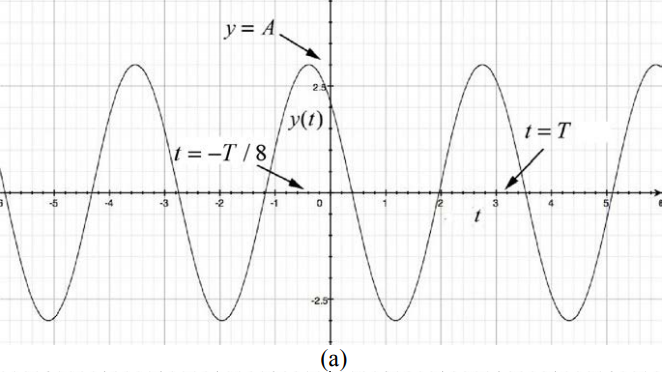
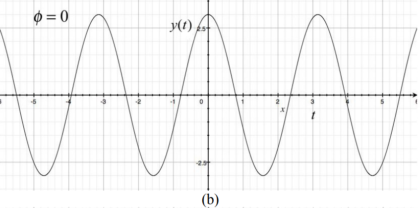
A plot of x t( ) vs. t is shown in Figure 23.4a with the values A=3,T=π and ϕ=π/4. Note that x(t)=Acos(ω0t+ϕ) takes on its maximum value when cos(ω0t+ϕ)=1. This occurs when ω0t+ϕ=2πn where n=0,±1,±2,⋯ The maximum value associated with n = 0 occurs when ω0t+ϕ=0 or t=−ϕ/ω0. For the case shown in Figure 23.4a where ϕ=π/4 this maximum occurs at the instant t=−T/8 Let’s plot x(t)=Acos(ω0t+ϕ) vs. t . Notice that when ϕ>0,x(t) is shifted to the left compared with the case ϕ=0 (compare Figures 23.4a with 23.4b). The function x(t)=Acos(ω0t+ϕ) with ϕ>0 reaches its maximum value at an earlier time than the function x(t)=Acos(ω0t). The difference in phases for these two cases is (ω0t+ϕ)−ω0t=ϕ and ϕ is sometimes referred to as the phase shift. When ϕ<0 the, function x(t)=Acos(ω0t+ϕ) reaches its maximum value at a later time t=T/8 than the function x(t)=Acos(ω0t) as shown in Figure 23.4c.

Example 23.2: Block-Spring System
A block of mass m is attached to a spring with spring constant k and is free to slide along a horizontal frictionless surface. At t = 0 , the block-spring system is stretched an amount x0>0 from the equilibrium position and is released from rest, vx,0=0. What is the period of oscillation of the block? What is the velocity of the block when it first comes back to the equilibrium position?
Solution: The position of the block can be determined from Equation (23.2.21) by substituting the initial conditions x0>0, and vx,0=0 yielding
x(t)=x0cos(√kmt)
and the x -component of its velocity is given by Equation (23.2.22),
vx(t)=−√kmx0sin(√kmt)
The angular frequency of oscillation is ω0=√k/m and the period is given by Equation (23.2.7),
T=2πω0=2π√mk
The block first reaches equilibrium when the position function first reaches zero. This occurs at time t1 satisfying
√kmt1=π2,t1=π2√mk=T4
The x -component of the velocity at time t1 is then
vx(t1)=−√kmx0sin(√kmt1)=−√kmx0sin(π/2)=−√kmx0=−ω0x0
Note that the block is moving in the negative x -direction at time t1; the block has moved from a positive initial position to the equilibrium position (Figure 23.4(b)).