
3.5: Linearly-damped Free Linear Oscillator


( \newcommand{\kernel}{\mathrm{null}\,}\)
General solution
All simple harmonic oscillations are damped to some degree due to energy dissipation via friction, viscous forces, or electrical resistance etc. The motion of damped systems is not conservative since energy is dissipated as heat. As was discussed in chapter 2 the damping force can be expressed as
FD(v)=−f(v)ˆv
where the velocity dependent function f(v) can be complicated. Fortunately there is a very large class of problems in electricity and magnetism, classical mechanics, molecular, atomic, and nuclear physics, where the damping force depends linearly on velocity which greatly simplifies solution of the equations of motion. Therefore this chapter will discuss linear damping.
Consider the free simple harmonic oscillator, that is, assuming no oscillatory forcing function, with a linear damping term FD(v)=−bv where the parameter b is the damping factor. Then the equation of motion is
−kx−b˙x=m¨x
This can be rewritten as
¨x+¨x+Γ˙x+ω20x=0
where the damping parameter
Γ=bm
and the characteristic angular frequency
ω0=√km
The general solution to the linearly-damped free oscillator is obtained by inserting the complex trial solution z=z0eiωt. Then
(iω)2z0eiωt+iωΓz0eiωt+ω20z0eiωt=0
This implies that
ω2−iωΓ−ω20=0
The solution is
ω±=iΓ2±√ω20−(Γ2)2
The two solutions ω± are complex conjugates and thus the solutions of the damped free oscillator are
z=z1ei(iΓ2+√ω20−(Γ2)2)t+z2ei(iΓ2−√ω20−(Γ2)2)t
This can be written as
z=e−(Γ2)t[z1eiω1t+z2e−iω1t]
where
ω1≡√ω2o−(Γ2)2
Underdamped motion ω21≡ω2o−(Γ2)2>0
When ω21>0 then the square root is real so the solution can be written taking the real part of z which gives that Equation ??? equals
x(t)=Ae−(Γ2)tcos(ω1t−β)
Where A and β are adjustable constants fit to the initial conditions. Therefore the velocity is given by
˙x(t)=−Ae−Γ2t[ω1sin(ω1t−β)+Γ2cos(ω1t−β)]
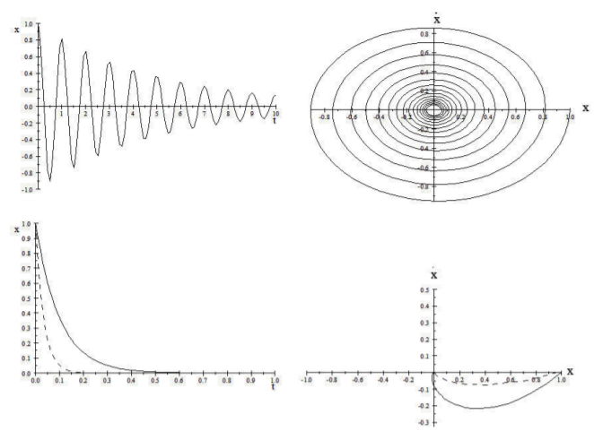
This is the damped sinusoidal oscillation illustrated in Figure 3.5.1-upper. The solution has the following characteristics:
- The oscillation amplitude decreases exponentially with a time constant τD=2Γ.
- There is a small reduction in the frequency of the oscillation due to the damping leading to ω1=√ω2o−(Γ2)2
Overdamped case ω21≡ω2o−(Γ2)2<0
In this case the square root of ω21 is imaginary and can be expressed as ω′1=i√(Γ2)2−ω2o. Therefore the solution is obtained more naturally by using a real trial solution z=z+0eωt in Equation ??? which leads to two roots
ω±=−[−Γ2±√(Γ2)2−ω2o]
Thus the exponentially damped decay has two time constants ω+ and ω−.
x(t)=A1e−ω+t+A2e−ω−t]
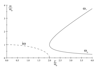
The time constant 1ω−<1ω+ thus the first term A1e−ω+t in the bracket decays in a shorter time than the second term A2e−ω−t. As illustrated in Figure 3.5.2 the decay rate, which is imaginary when underdamped, i.e. Γ2<ωo bifurcates into two real values ω± for overdamped, i.e. Γ2>ωo. At large times the dominant term when overdamped is for ω+ which has the smallest decay rate, that is, the longest decay constant τ+=1ω+. There is no oscillatory motion for the overdamped case, it slowly moves monotonically to zero as shown in fig 3.5 lower. The amplitude decays away with a time constant that is longer than 2Γ.
Critically damped ω21≡ω2o−(Γ2)2=0
This is the limiting case where Γ2=ωo For this case the solution is of the form
x(t)=(A+Bt)e−(Γ2)t
This motion also is non-sinusoidal and evolves monotonically to zero. As shown in Figure 3.5.1 the critically-damped solution goes to zero with the shortest time constant, that is, largest ω. Thus analog electric meters are built almost critically damped so the needle moves to the new equilibrium value in the shortest time without oscillation.
It is useful to graphically represent the motion of the damped linear oscillator on either a state space (˙x,x) diagram or phase space (px,x) diagram as discussed in chapter 3.4. The state space plots for the undamped, overdamped, and critically-damped solutions of the damped harmonic oscillator are shown in Figure 3.5.1. For underdamped motion the state space diagram spirals inwards to the origin in contrast to critical or overdamped motion where the state and phase space diagrams move monotonically to zero.
Energy dissipation
The instantaneous energy is the sum of the instantaneous kinetic and potential energies
E=12m˙x2+12kx2
where x and ˙x are given by the solution of the equation of motion. Consider the total energy of the underdamped system
E=12m˙x2+12mω20x2
where k=mω20. The average total energy is given by substitution for x and ˙x and taking the average over one cycle. Since
x(t)=Ae−(Γ2)tcos(ω1t−β)
Then the velocity is given by
˙x(t)=−Ae−Γ2t[ω1sin(ω1t−β)+Γ2cos(ω1t−β)]
Inserting equations ??? and ??? into ??? gives a small amplitude oscillation about an exponential decay for the energy E. Averaging over one cycle and using the fact that ⟨sinθcosθ⟩=0, and ⟨[sinθ]2⟩=⟨[cosθ]2⟩=12, gives the time-averaged total energy as
⟨E⟩=e−Γt(14mA2ω21+14mA2(Γ2)2+14mA2ω20)
which can be written as
⟨E⟩=E0e−Γt
Note that the energy of the linearly damped free oscillator decays away exponentially with a time constant τ=1Γ. That is, the intensity has a time constant that is half the time constant for the decay of the amplitude of the transient response. Note that the average kinetic and potential energies are identical, as implied by the Virial theorem, and both decay away with the same time constant. This relation between the mean life τ for decay of the damped harmonic oscillator and the damping width term Γ occurs frequently in physics.
The damping of an oscillator usually is characterized by a single parameter Q called the Quality Factor where
Q≡Energy stored in the oscillatorEnergy dissipated per radian
The energy loss per radian is given by
ΔE=dEdt1ω1=EΓω1=EΓ√ω2o−(Γ2)2
where the numerator ω1=√ω2o−(Γ2)2 is the frequency of the free damped linear oscillator.
Thus the Quality factor Q equals
Q=EΔE=ω1Γ
The larger the Q factor, the less damped is the system, and the greater is the number of cycles of the oscillation in the damped wave train. Chapter 3.11.3 shows that the longer the wave train, that is the higher is the Q factor, the narrower is the frequency distribution around the central value. The Mössbauer effect in nuclear physics provides a remarkably long wave train that can be used to make high precision measurements. The high-Q precision of the LIGO laser interferometer was used in the recent successful search for gravity waves.
| Oscillating system | Typical Q factors |
|---|---|
| Earth, for earthquake wave | 250-1400 |
| Piano string | 3000 |
| Crystal in digital watch | 104 |
| Microwave cavity | 104 |
| Excited atom | 107 |
| Neutron star | 1012 |
| LIGO laser | 1013 |
| Mössbauer effect in nucleus | 1014 |