3.6: Sinusoidally-driven, linearly-damped, linear oscillator


- Last updated
- Mar 14, 2021
- Save as PDF

( \newcommand{\kernel}{\mathrm{null}\,}\)
The linearly-damped linear oscillator, driven by a harmonic driving force, is of considerable importance to all branches of science and engineering. The equation of motion can be written as
¨x+Γ˙x+w20x=F(t)m
where F(t) is the driving force. For mathematical simplicity the driving force is chosen to be a sinusoidal harmonic force. The solution of this second-order differential equation comprises two components, the complementary solution (transient response), and the particular solution (steady-state response).
Transient response of a driven oscillator
The transient response of a driven oscillator is given by the complementary solution of the above second-order differential equation
¨x+Γ˙x+ω20x=0
which is identical to the solution of the free linearly-damped harmonic oscillator. As discussed in section 3.5 the solution of the linearly-damped free oscillator is given by the real part of the complex variable z where
z=e−Γ2t[z1eiω1t+z2e−iω1t]
and
ω1≡√ω2o−(Γ2)2
Underdamped motion ω21≡ω2o−Γ22>0:
When ω21>0, then the square root is real so the transient solution can be written taking the real part of z which gives
x(t)T=F0me−Γ2tcos(ω1t)
The solution has the following characteristics:
a) The amplitude of the transient solution decreases exponentially with a time constant τD=2Γ while the energy decreases with a time constant of 1Γ.
b) There is a small downward frequency shift in that ω1=√ω2o−(Γ2)2.
Overdamped case ω21≡ω2o−(Γ2)2<0:
In this case the square root is imaginary, which can be expressed as ω′1≡√(Γ2)2−ω2o which is real and the solution is just an exponentially damped one
x(t)T=F0me−Γ2t[eω′1t+e−ω′1t]
There is no oscillatory motion for the overdamped case, it slowly moves monotonically to zero. The total energy decays away with two time constants greater than 1Γ.
Critically damped ω21≡ω2o−(Γ2)2=0:
For this case, as mentioned for the damped free oscillator, the solution is of the form
x(t)T=(A+Bt)e−Γ2t
The critically-damped system decays away the quickest.
Steady state response of a driven oscillator
The particular solution of the differential equation gives the important steady state response, x(t)S to the forcing function. Consider that the forcing term is a single frequency sinusoidal oscillation.
F(t)=F0cos(ωt)
Thus the particular solution is the real part of the complex variable z which is a solution of
¨z+Γ˙z+ω20z=F0meiωt
A trial solution is
z=z0eiωt
This leads to the relation
−ω2z0+iωΓz0+ω20z0=F0m
Multiplying the numerator and denominator by the factor (ω20−ω2)−iΓω gives
z0=F0m(ω20−ω2)+iΓω=F0m(ω20−ω2)2+(Γω)2[(ω20−ω2)−iΓω]
The steady state solution x(t)S thus is given by the real part of z, that is
x(t)S=F0m(ω20−ω2)2+(Γω)2[(ω20−ω2)cosωt+Γωsinωt]
This can be expressed in terms of a phase δ defined as
tanδ≡(Γωω20−ω2)
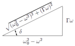
As shown in Figure 3.6.1 the hypotenuse of the triangle equals √(ω20−ω2)2+(Γω)2. Thus
cosδ=ω20−ω2√(ω20−ω2)2+(Γω)2
and
sinδ=Γω√(ω20−ω2)2+(Γω)2
The phase δ represents the phase difference between the driving force and the resultant motion. For a fixed ω0 the phase δ=0 when ω=0, and increases to δ=π2 when ω=ω0. For ω>ω0 the phase δ→π as ω→∞.
The steady state solution can be re-expressed in terms of the phase shift δ as
x(t)S=F0m√(ω20−ω2)2+(Γω)2[cosδcosωt+sinδsinωt]=F0m√(ω20−ω2)2+(Γω)2cos(ωt−δ)
Complete solution of the driven oscillator
To summarize, the total solution of the sinusoidally forced linearly-damped harmonic oscillator is the sum of the transient and steady-state solutions of the equations of motion.
x(t)Total=x(t)T+x(t)S
This for the underdamped case, the transient solution is the complementary solution
x(t)T=F0me−Γ2tcos(ω1t−β)
where ω1=√ω2o−(Γ2)2. The steady-state solution is given by the particular solution
x(t)S=F0m√(ω20−ω2)2+(Γω)2cos(ωt−δ)
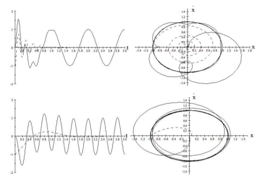
Note that the frequency of the transient solution is ω1 which in general differs from the driving frequency ω. The phase shift β−δ for the transient component is set by the initial conditions. The transient response leads to a more complicated motion immediately after the driving function is switched on. Figure 3.6.2 illustrates the amplitude time dependence and state space diagram for the transient component, and the total response, when the driving frequency is either ω=ω15 or ω=5ω1. Note that the modulation of the steady-state response by the transient response is unimportant once the transient response has damped out leading to a constant elliptical state space trajectory. For cases where the initial conditions are x=˙x=0 then the transient solution has a relative phase difference β−δ=π radians at t=0 and relative amplitudes such that the transient and steady-state solutions cancel at t=0.
The characteristic sounds of different types of musical instruments depend very much on the admixture of transient solutions plus the number and mixture of oscillatory active modes. Percussive instruments, such as the piano, have a large transient component. The mixture of transient and steady-state solutions for forced oscillations occurs frequently in studies of RLC networks in electrical circuit analysis.
Resonance
The discussion so far has discussed the role of the transient and steady-state solutions of the driven damped harmonic oscillator which occurs frequently is science, and engineering. Another important aspect is resonance that occurs when the driving frequency ω approaches the natural frequency ω1 of the damped system. Consider the case where the time is sufficient for the transient solution to have decayed to zero.
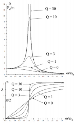
Figure 3.6.3 shows the amplitude and phase for the steady-state response as ω goes through a resonance as the driving frequency is changed. The steady-states solution of the driven oscillator follows the driving force when ω<<ω0 in that the phase difference is zero and the amplitude is just F0k. The response of the system peaks at resonance, while for ω>>ω0 the harmonic system is unable to follow the more rapidly oscillating driving force and thus the phase of the induced oscillation is out of phase with the driving force and the amplitude of the oscillation tends to zero.
Note that the resonance frequency for a driven damped oscillator, differs from that for the undriven damped oscillator, and differs from that for the undamped oscillator. The natural frequency for an undamped harmonic oscillator is given by
ω20=km
The transient solution is the same as damped free oscillations of a damped oscillator and has a frequency of the system ω1 given by
ω21=ω20−(Γ2)2
That is, damping slightly reduces the frequency.
For the driven oscillator the maximum value of the steady-state amplitude response is obtained by taking the maximum of the function x(t)s, that is when dxSdω=0. This occurs at the resonance angular frequency ωR where
ω2R=ω20−2(Γ2)2
No resonance occurs if ω20−2(Γ2)2<0 since then ωR is imaginary and the amplitude decreases monotonically with increasing ω. Note that the above three frequencies are identical if Γ=0 but they differ when Γ>0 with ωR<ω1<ω0.
For the driven oscillator it is customary to define the quality factor Q as
Q≡ωRΓ
When Q>>1 then one has a narrow high resonance peak. As the damping increases the quality factor decreases leading to a wider and lower peak. The resonance disappears when Q<1.
Energy absorption
Discussion of energy stored in resonant systems is best described using the steady state solution which is dominant after the transient solution has decayed to zero. Then
x(t)S=F0m(ω20−ω2)2+(Γω)2[(ω20−ω2)cosωt+Γωsinωt]
This can be rewritten as
x(t)S=Aelcosωt+Aabssinωt
where the elastic amplitude
Ael=F0m(ω20−ω2)2+(Γω)2(ω20−ω2)
while the absorptive amplitude
Aabs=F0m(ω20−ω2)2+(Γω)2Γω
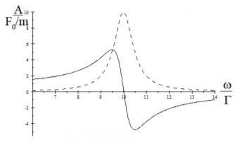
Figure 3.6.4 shows the behavior of the absorptive and elastic amplitudes as a function of angular frequency ω. The absorptive amplitude is significant only near resonance whereas the elastic amplitude goes to zero at resonance. Note that the full width at half maximum of the absorptive amplitude peak equals Γ.
The work done by the force F0cosωt on the oscillator is
W=∫Fdx=∫F˙xdt
Thus the absorbed power P(t) is given by
P(t)=dWdt=F˙x
The steady state response gives a velocity
˙x(t)S=−ωAelsinωt+ωAabscosωt
Thus the steady-state instantaneous power input is
P(t)=F0cosωt[−ωAelsinωt+ωAabscosωt]
The absorptive term steadily absorbs energy while the elastic term oscillates as energy is alternately absorbed or emitted. The time average over one cycle is given by
⟨P⟩=F0[−ωAel⟨cosωtsinωt⟩+ωAabs⟨(cosωt)2⟩]
where ⟨cosωtsinωt⟩ and ⟨cosωt2⟩ are the time average over one cycle. The time averages over one complete cycle for the first term in the bracket is
−ωAel⟨cosωtsinωt⟩=0
while for the second term
⟨cosωt2⟩=1T∫t0+Ttocosωt2dt=12
Thus the time average power input is given by only the absorptive term
⟨P⟩=12F0ωAabs=F202mΓω2(ω20−ω2)2+(Γω)2
This shape of the power curve is a classic Lorentzian shape. Note that the maximum of the average kinetic energy occurs at ωKE=ω0 which is different from the peak of the amplitude which occurs at ω21=ω20−(Γ2)2. The potential energy is proportional to the amplitude squared, i.e. x2S which occurs at the same angular frequency as the amplitude, that is, ω2PE=ω2R=ω20−2(Γ2)2. The kinetic and potential energies resonate at different angular frequencies as a result of the fact that the driven damped oscillator is not conservative because energy is continually exchanged between the oscillator and the driving force system in addition to the energy dissipation due to the damping.
When ω∼ω0>>Γ, then the power equation simplifies since
(ω20−ω2)=(ω0+ω)(ω0−ω)≈2ω0(ω0−ω)
Therefore
⟨P⟩≃F208mΓ(ω0−ω)2+(Γ2)2
This is called the Lorentzian or Breit-Wigner shape. The half power points are at a frequency difference from resonance of ±Δω where
Δω=|ω0−ω|=±Γ2
Thus the full width at half maximum of the Lorentzian curve equals Γ. Note that the Lorentzian has a narrower peak but much wider tail relative to a Gaussian shape. At the peak of the absorbed power, the absorptive amplitude can be written as
Aabs(ω=ω0)=F0mQω20
That is, the peak amplitude increases with increase in Q. This explains the classic comedy scene where the soprano shatters the crystal glass because the highest quality crystal glass has a high Q which leads to a large amplitude oscillation when she sings on resonance.
The mean lifetime τ of the free linearly-damped harmonic oscillator, that is, the time for the energy of free oscillations to decay to 1/e was shown to be related to the damping coefficient Γ by
τ=1Γ
Therefore we have the classical uncertainty principle for the linearly-damped harmonic oscillator that the measured full-width at half maximum of the energy resonance curve for forced oscillation and the mean life for decay of the energy of a free linearly-damped oscillator are related by
τΓ=1
This relation is correct only for a linearly-damped harmonic system. Comparable relations between the lifetime and damping width exist for different forms of damping.
One can demonstrate the above line width and decay time relationship using an acoustically driven electric guitar string. It also occurs for the width of the electromagnetic radiation and the lifetime for decay of atomic or nuclear electromagnetic decay. This classical uncertainty principle is exactly the same as the one encountered in quantum physics due to wave-particle duality. In nuclear physics it is difficult to measure the lifetime of states when τ<10−13s. For shorter lifetimes the value of Γ can be determined from the shape of the resonance curve which can be measured directly when the damping is large.
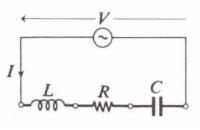
Example 3.6.1: Harmonically-driven series RLC circuit
The harmonically-driven, resonant, series RLC circuit, is encountered frequently in AC circuits. Kirchhoff’s Rules applied to the series RLC circuit lead to the differential equation
L¨q+R˙q+qC=V0sinωt
where q is charge, L is the inductance, C is the capacitance, R is the resistance, and the applied voltage across the circuit is V(ω)=V0sinωt. The linearity of the network allows use of the phasor approach which assumes that the current I=I0eiωt, the voltage V=V0ei(ωt+δ), and the impedance is a complex number Z=V0I0eiδ where δ is the phase difference between the voltage and the current. For this circuit the impedance is given by
Z=R+i(ωL−1ωC)
Because of the phases involved in this RLC circuit, at resonance the maximum voltage across the resistor occurs at a frequency of ωR=ω0, across the capacitor the maximum voltage occurs at a frequency ω2C=ω20−R22L2, and across the inductor L the maximum voltage occurs at a frequency ω2L=ω201−R22L2, where ω20=1LC is the resonance angular frequency when R=0. Thus these resonance frequencies differ when R>0.