5.2: Projectile Motion

Consider the motion of a body that is released at time t = 0 with an initial velocity \(\overrightarrow{\mathbf{v}}_{0}\). Two paths are shown in Figure 5.1.

Figure 5.1 Actual orbit accounting for air resistance and parabolic orbit of a projectile

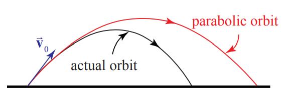
The dotted path represents a parabolic trajectory and the solid path represents the actual trajectory. The difference between the two paths is due to air resistance acting on the object, \(\overrightarrow{\mathbf{F}}^{a i r}=-b v^{2} \hat{\mathbf{v}}\), where \(\hat{\mathbf{v}}\) is a unit vector in the direction of the velocity. (For the orbits shown in Figure \(5.1, b=0.01 \mathrm{N} \cdot \mathrm{s}^{2} \cdot \mathrm{m}^{-2}\), \(\left|\overrightarrow{\mathbf{v}}_{0}\right|=30.0 \mathrm{m} \cdot \mathrm{s}\), the initial launch angle with respect to the horizontal \(\theta_{0}=21^{\circ}\) and the actual horizontal distance traveled is \(71.7 \%\) of the projectile orbit.). There are other factors that can influence the path of motion; a rotating body or a special shape can alter the flow of air around the body, which may induce a curved motion or lift like the flight of a baseball or golf ball. We shall begin our analysis by neglecting all interactions except the gravitational interaction.

Figure 5.2 A coordinate sketch for parabolic motion.

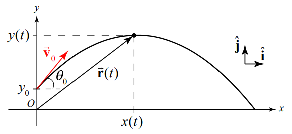
Choose coordinates with the positive y-axis in the upward vertical direction and the positive x-axis in the horizontal direction in the direction that the object is moving horizontally. Choose the origin at the ground immediately below the point the object is released. Figure 5.2 shows our coordinate system with the position of the object \(\overrightarrow{\mathbf{r}}(t)\) at time t , the initial velocity \(\overrightarrow{\mathbf{v}}_{0}\), and the initial angle \(\theta_{0}\) with respect to the horizontal, and the coordinate functions x(t) and y(t).

Initial Conditions:

Figure 5.3 A vector decomposition of the initial velocity

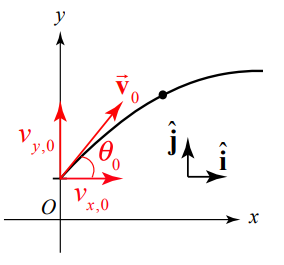
Decompose the initial velocity vector into its components:

\[\overrightarrow{\mathbf{v}}_{0}=v_{x, 0} \hat{\mathbf{i}}+v_{y, 0} \hat{\mathbf{j}} \nonumber \]

The vector decomposition for the initial velocity is shown in Figure 5.3. Often the description of the flight of a projectile includes the statement, “a body is projected with an initial speed \(v_{0}\) at an angle \(\theta_{0}\) with respect to the horizontal.” The components of the initial velocity can be expressed in terms of the initial speed and angle according to

\[v_{x, 0}=v_{0} \cos \theta_{0} \nonumber \]

\[v_{y, 0}=v_{0} \sin \theta_{0} \nonumber \]

Because the initial speed is the magnitude of the initial velocity, we have that

\[v_{0}=\left(v_{x, 0}^{2}+v_{y, 0}^{2}\right)^{1 / 2} \nonumber \]

The angle \(\theta_{0}\) is related to the components of the initial velocity by

\[\theta_{0}=\tan ^{-1}\left(v_{y, 0} / v_{x, 0}\right) \nonumber \]

Equation (5.1.8) will give two values for the angle \(\theta_{0}\), so care must be taken to choose the correct physical value. The initial position vector generally is given by

\[\overrightarrow{\mathbf{r}}_{0}=x_{0} \hat{\mathbf{i}}+y_{0} \hat{\mathbf{j}} \nonumber \]

Note that the trajectory in Figure 5.3 has \(x_{0}=0\), but this will not always be the case.

Force Diagram

We begin by neglecting all forces other than the gravitational interaction between the object and the earth. This force acts downward with magnitude mg , where m is the mass of the object and \(g=9.8 \mathrm{m} \cdot \mathrm{s}^{-2}\). Figure 5.4 shows the force diagram on the object.

Figure 5.4 Free-body force diagram on the object with the action of gravity

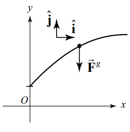
The vector decomposition of the force is

\[\overrightarrow{\mathbf{F}}^{g}=-m g \hat{\mathbf{j}} \nonumber \]

Equations of Motions

The force diagram reminds us that the force is acting in the y -direction. Newton’s Second Law states that the sum of the force, \(\overrightarrow{\mathbf{F}}^{\text {total }}\), acting on the object is equal to the product of the mass m and the acceleration vector \(\overrightarrow{\mathbf{a}}\)

\[\overrightarrow{\mathbf{F}}^{\text {total }}=m \overrightarrow{\mathbf{a}} \nonumber \]

Because we are modeling the motion with only one force, we have that \(\overrightarrow{\mathbf{F}}^{\text {total }}=\overrightarrow{\mathbf{F}}^{g}\). This is a vector equation; the components are equated separately:

\[-m g=m a_{y} \nonumber \]

\[0=m a_{x} \nonumber \]

Therefore the y -component of the acceleration is

\[a_{y}=-g \nonumber \]

We see that the acceleration is a constant and is independent of the mass of the object. Notice that \(a_{y}<0\). This is because we chose our positive y -direction to point upwards. The sign of the y -component of acceleration is determined by how we choose our coordinate system. Because there are no horizontal forces acting on the object, we conclude that the acceleration in the horizontal direction is also zero

\[a_{x}=0 \nonumber \]

Therefore the x -component of the velocity remains unchanged throughout the flight of the object.

The acceleration in the vertical direction is constant for all bodies near the surface of the Earth, independent of the mass of the object, thus confirming Galileo’s Law of Free Falling Bodies. Notice that the equation of motion (Equation (5.1.14)) generalizes the experimental observation that objects fall with constant acceleration. Our statement about the acceleration of objects near the surface of Earth depends on our model force law Equation (5.1.10), and if subsequent observations show the acceleration is not constant then we either must include additional forces (for example, air resistance), or modify the force law (for objects that are no longer near the surface of Earth, or consider that Earth is a non-symmetric non-uniform body), or take into account the rotational motion of the Earth.

We can now integrate the equation of motions (Equations (5.1.14) and (5.1.15)) separately for the x - and y - directions to find expressions for the x - and y -components of velocity and position:

\[\begin{align}
v_{x}(t)-v_{x, 0} &=\int_{t^{\prime}=0}^{t^{\prime}=t} a_{x}\left(t^{\prime}\right) d t^{\prime}=0 \Rightarrow v_{x}(t)=v_{x, 0} \\[4pt]
x(t)-x_{0}&=\int_{t^{\prime}=0}^{t^{\prime}=t} v_{x}\left(t^{\prime}\right) d t^{\prime} =\int_{t^{\prime}=0}^{t^{\prime}=t} v_{x, 0} d t^{\prime}=v_{x, 0} t \Rightarrow x(t)=x_{0}+v_{x, 0} t \\[4pt]
v_{y}(t)-v_{y, 0} &=\int_{t^{\prime}=0}^{t^{\prime}=t} a_{y}\left(t^{\prime}\right) d t^{\prime}=-\int_{t^{\prime}=0}^{t^{\prime}=t} g d t^{\prime}=-g t \Rightarrow v_{y}(t)=v_{y, 0}-g t \\[4pt]
y(t)-y_{0}&=\int_{t=0}^{t=t} v_{y}\left(t^{\prime}\right) d t^{\prime}=\int_{t^{\prime}=0}^{t=t}\left(v_{y, 0}-g t\right) d t^{\prime}=v_{y, 0} t-(1 / 2) g t^{2} \Rightarrow y(t)=y_{0}+v_{y, 0} t-(1 / 2) g t^{2}
\end{align} \nonumber \]

The complete set of vector equations for position and velocity for each independent direction of motion are given by

\[\overrightarrow{\mathbf{r}}(t)=x(t) \hat{\mathbf{i}}+y(t) \hat{\mathbf{j}}=\left(x_{0}+v_{x, 0} t\right) \hat{\mathbf{i}}+\left(y_{0}+v_{y, 0} t+(1 / 2) a_{y} t^{2}\right) \hat{\mathbf{j}} \nonumber \]

\[\overrightarrow{\mathbf{v}}(t)=v_{x}(t) \hat{\mathbf{i}}+v_{y}(t) \hat{\mathbf{j}}=v_{x, 0} \hat{\mathbf{i}}+\left(v_{y, 0}+a_{y} t\right) \hat{\mathbf{j}} \nonumber \]

\[\overrightarrow{\mathbf{a}}(t)=a_{x}(t) \hat{\mathbf{i}}+a_{y}(t) \hat{\mathbf{j}}=a_{y} \hat{\mathbf{j}} \nonumber \]

Example \(\PageIndex{1}\): Time of Flight and Maximum Height of a Projectile

A person throws a stone at an initial angle \(\theta_{0}=45^{\circ}\) from the horizontal with an initial speed of \(v_{0}=20 \mathrm{m} \cdot \mathrm{s}^{-1}\). The point of release of the stone is at a height d = 2 m above the ground. You may neglect air resistance. a) How long does it take the stone to reach the highest point of its trajectory? b) What was the maximum vertical displacement of the stone? Ignore air resistance.

Solution: Choose the origin on the ground directly underneath the point where the stone is released. We choose the positive y-axis in the upward vertical direction and the positive x-axis in the horizontal direction in the direction that the object is moving horizontally. Set t = 0 the instant the stone is released. At t = 0 the initial conditions are then \(x_{0}=0\) and \(y_{0}=d\). The initial x - and y -components of the velocity are given by Equations (5.1.5) and (5.1.6).

At time t the stone has coordinates (x(t), y(t)) . These coordinate functions are shown in Figure 5.5.

Figure 5.5: Coordinate functions for stone

Figure 5.6 Plot of the y-component of the position as a function of time

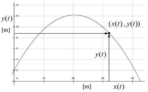
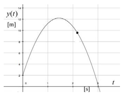
The slope of this graph at any time t yields the instantaneous y-component of the velocity \(v_{y}(t)\) at that time t . Figure 5.5 is a plot of y(t) vs. x(t) and Figure 5.6 is a plot of y(t) vs. t . There are several important things to notice about Figures 5.5 and 5.6. The first point is that the abscissa axes are different in both figures. The second thing to notice is that at t = 0 , the slope of the graph in Figure 5.5 is equal to

\[\left.\frac{d y}{d x}\right|_{t=0}=\left.\left(\frac{d y / d t}{d x / d t}\right)\right|_{t=0}=\frac{v_{y, 0}}{v_{x, 0}}=\tan \theta_{0} \nonumber \]

while at t = 0 the slope of the graph in Figure 5.6 is equal to

\[\left.\frac{d y}{d t}\right|_{t=0}=v_{y, 0} \nonumber \]

The slope of this graph in Figure 5.6 at any time t yields the instantaneous y-component of the velocity \(v_{y}(t)\) at that time t . Let \(t=t_{1}\) correspond to the instant the stone is at its maximal vertical position, the highest point in the flight. The final thing to notice about Figure 5.6 is that a \(t=t_{1}\) the slope is zero or \(v_{y}\left(t=t_{1}\right)=0\). Therefore

\[v_{y}\left(t_{1}\right)=v_{0} \sin \theta_{0}-g t_{1}=0 \nonumber \]

Solving Equation (5.1.21) for \(t_{1}\) yields,

\[t_{1}=\frac{v_{0} \sin \theta_{0}}{g}=\frac{\left(20 \mathrm{m} \cdot \mathrm{s}^{-1}\right) \sin \left(45^{\circ}\right)}{9.8 \mathrm{m} \cdot \mathrm{s}^{-2}}=1.44 \mathrm{s} \nonumber \]

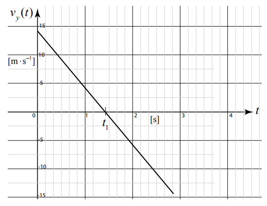
The graph in Figure 5.7 shows a plot of \(v_{y}(t)\) as a function of time. Notice that at t = 0 the intercept is positive indicting that \(\mathcal{V}_{y, 0}\) is positive which means that the stone was thrown upwards. The y -component of the velocity changes sign at \(t=t_{1}\) indicating that the stone is reversing its direction and starting to move downwards.

Figure 5.7 y -component of the velocity as a function of time

We now substitute the expression for \(t=t_{t o p}\) (Equation (5.1.22)) into the y -component of the position in Equation (5.1.16) to find the maximal height of the stone above the ground

\[\begin{array}{l}
y\left(t=t_{t o p}\right)=d+v_{0} \sin \theta_{0} \frac{v_{0} \sin \theta_{0}}{g}-\frac{1}{2} g\left(\frac{v_{0} \sin \theta_{0}}{g}\right)^{2} \\
=d+\frac{v_{0}^{2} \sin ^{2} \theta_{0}}{2 g}=2 \mathrm{m}+\frac{\left(20 \mathrm{m} \cdot \mathrm{s}^{-1}\right)^{2} \sin ^{2}\left(45^{\circ}\right)}{2\left(9.8 \mathrm{m} \cdot \mathrm{s}^{-2}\right)}=12.2 \mathrm{m}
\end{array} \nonumber \]

Orbit Equation

So far our description of the motion has emphasized the independence of the spatial dimensions, treating all of the kinematic quantities as functions of time. We shall now eliminate time from our equation and find the orbit equation of the body undergoing projectile motion. We begin with the x -component of the position in Equation (5.1.16),

\[x(t)=x_{0}+v_{x, 0} t \nonumber \]

and solve Equation (5.1.24) for time t as a function of x(t),

\[t=\frac{x(t)-x_{0}}{v_{x, 0}} \nonumber \]

The y -component of the position in Equation (5.1.16) is given by

\[y(t)=y_{0}+v_{y, 0} t-\frac{1}{2} g t^{2} \nonumber \]

We then substitute Equation (5.1.25) into Equation (5.1.26) yielding

\[y(t)=y_{0}+v_{y, 0}\left(\frac{x(t)-x_{0}}{v_{x, 0}}\right)-\frac{1}{2} g\left(\frac{x(t)-x_{0}}{v_{x, 0}}\right)^{2} \nonumber \]

A little algebraic simplification yields the equation for a parabola:

\[y(t)=-\frac{1}{2} \frac{g}{v_{x, 0}^{2}} x(t)^{2}+\left(\frac{g x_{0}}{v_{x, 0}^{2}}+\frac{v_{y, 0}}{v_{x, 0}}\right) x(t)-\frac{v_{y, 0}}{v_{x, 0}} x_{0}-\frac{1}{2} \frac{g}{v_{x, 0}^{2}} x_{0}^{2}+y_{0} \nonumber \]

The graph of y(t) as a function of x(t) is shown in Figure 5.8.

Figure 5.8 The parabolic orbit

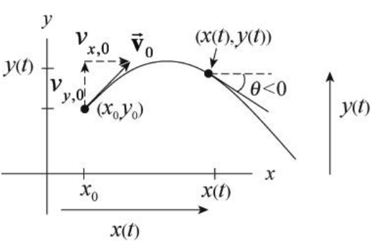
The velocity vector is given by

\[\overrightarrow{\mathbf{v}}(t)=\frac{d x(t)}{d t} \hat{\mathbf{i}}+\frac{d y(t)}{d t} \hat{\mathbf{j}} \equiv v_{x}(t) \hat{\mathbf{i}}+v_{y}(t) \hat{\mathbf{j}} \nonumber \]

The direction of the velocity vector at a point (x(t), y(t)) can be determined from the components. Let θ be the angle that the velocity vector forms with respect to the positive x -axis. Then

\[\theta=\tan ^{-1}\left(\frac{v_{y}(t)}{v_{x}(t)}\right)=\tan ^{-1}\left(\frac{d y / d t}{d x / d t}\right)=\tan ^{-1}\left(\frac{d y}{d x}\right) \nonumber \]

Differentiating Equation (5.1.28) with respect to x yields

\[\frac{d y}{d x}=-\frac{g}{v_{x, 0}^{2}} x+\left(\frac{g x_{0}}{v_{x, 0}^{2}}+\frac{v_{y, 0}}{v_{x, 0}}\right) \nonumber \]

The direction of the velocity vector at a point (x(t), y(t)) is therefore

\[\theta=\tan ^{-1}\left(-\frac{g}{v_{x, 0}^{2}} x+\left(\frac{g x_{0}}{v_{x, 0}^{2}}+\frac{v_{y, 0}}{v_{x, 0}}\right)\right) \nonumber \]

Although we can determine the angle of the velocity, we cannot determine how fast the body moves along the parabolic orbit from our graph of y(x) ; the magnitude of the velocity cannot be determined from information about the tangent line.

If we choose our origin at the initial position of the body at t = 0 , then \(x_{0}=0\) and \(y_{0}=0\). Our orbit equation, Equation (5.1.28) can now be simplified to

\[y(t)=-\frac{1}{2} \frac{g}{v_{x, 0}^{2}} x(t)^{2}+\frac{v_{y, 0}}{v_{x, 0}} x(t) \nonumber \]

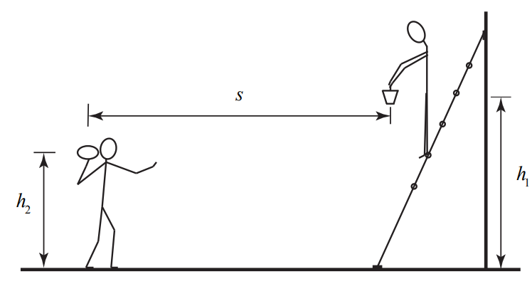
Example \(\PageIndex{2}\): Hitting the Bucket

A person is holding a pail while standing on a ladder. The person releases the pail from rest at a height \(h_{1}\), above the ground. A second person, standing a horizontal distance s from the pail, aims and throws a ball the instant the pail is released in order to hit the pail. The person releases the ball at a height \(h_{2}\) above the ground, with an initial speed \(v_{0}\), and at an angle \(\theta_{0}\) with respect to the horizontal. Assume that \(v_{0}\) is large enough so that the stone will at least travel a horizontal distance s before it hits the ground. You may ignore air resistance.

Figure 5.9: Example 5.2

1. Find an expression for the angle \(\theta_{0}\) that the person aims the ball in order to hit the pail. Does the answer depend on the initial velocity?
2. Find an expression for the time of collision as a function of the initial speed of the ball \(\v_{0}\), and the quantities \(\h_{1}\), \(\h_{2}\), and s .
3. Find an expression for the height above the ground where the collision occurred as a function of the initial speed of the ball \(\v_{0}\), and the quantities \(\h_{1}\), \(\h_{2}\), and s.

Solution

There are two objects involved in this problem. Each object is undergoing free fall, so there is only one stage of motion for each object. The pail is undergoing one-dimensional motion. The ball is undergoing two-dimensional motion. The parameters \(\h_{1}\), \(\h_{2}\), \(\v_{0}\), and s are unspecified, so our answers will be functions of those quantities. Figure 5.9 shows a sketch of the motion of all the bodies in this problem.

Choose an origin on the ground directly underneath the point where the ball is released, upwards for the positive y -direction and towards the pail for the positive x -direction. Choose position coordinates for the pail as follows. The horizontal coordinate is constant and given by \(x_{1}=s\). The vertical coordinate represents the height above the ground and is denoted by \(y_{1}(t)\). The ball has coordinates \(\left(x_{2}(t), y_{2}(t)\right)\). We show these coordinates in the Figure 5.10.

Figure 5.10: Coordinate System

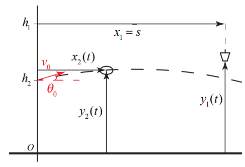
The pail undergoes constant acceleration \(a_{1, y}=-g\) in the vertical direction and the ball undergoes uniform motion in the horizontal direction and constant acceleration in the vertical direction, with \(a_{2, x}=0\) and \(a_{2, y}=-g\).

The initial conditions for the pail are \(\left(v_{1,0}\right)_{y}=0, x_{1,0}=s, y_{1,0}=h_{1}\). The equations for position and velocity of the pail simplify to

\[y_{1}(t)=h_{1}-\frac{1}{2} g t^{2} \nonumber \]

\[v_{y, 1}(t)=-g t \nonumber \]

The initial position is given by \(x_{2,0}=0, y_{2,0}=h_{2}\). The components of the initial velocity are given by \(\left(v_{2,0}\right)_{y}=v_{0} \sin \left(\theta_{0}\right)\) and \(\left(v_{2,0}\right)_{x}=v_{0} \cos \left(\theta_{0}\right)\), where \(v_{0}\) is the magnitude of the initial velocity and \(\theta_{0}\) is the initial angle with respect to the horizontal. The equations for the position and velocity of the ball simplify to

\[x_{2}(t)=v_{0} \cos \left(\theta_{0}\right) t \nonumber \]

\[v_{2 x}(t)=v_{0} \cos \left(\theta_{0}\right) \nonumber \]

\[y_{2}(t)=h_{2}+v_{0} \sin \left(\theta_{0}\right) t-\frac{1}{2} g t^{2} \nonumber \]

\[v_{2, y}(t)=v_{0} \sin \left(\theta_{0}\right)-g t \nonumber \]

Note that the quantities \(h_{1}, h_{2}, v_{0}\), and s should be treated as known quantities although no numerical values were given. There are six independent equations with 8 as yet unspecified quantities \(y_{1}(t), t, y_{2}(t), x_{2}(t), v_{1, y}(t), v_{2, y}(t), v_{2, x}(t)\), and \(\theta_{0}\).

So we need two more conditions, in order to find expressions for the initial angle, \(\theta_{0}\), the time of collision, \(t_{a}\), and the spatial location of the collision point specified by \(y_{1}\left(t_{a}\right)\) or \(y_{2}\left(t_{a}\right)\). At the collision time \(t=t_{a}\) the collision occurs when the two balls are located at the same position. Therefore

\[y_{1}\left(t_{a}\right)=y_{2}\left(t_{a}\right) \nonumber \]

\[x_{2}\left(t_{a}\right)=x_{1}=s \nonumber \]

We shall now apply these conditions that must be satisfied in order for the ball to hit the pail.

\[h_{1}-\frac{1}{2} g t_{a}^{2}=h_{2}+v_{0} \sin \left(\theta_{0}\right) t_{a}-\frac{1}{2} g t_{a}^{2} \nonumber \]

\[s=v_{0} \cos \left(\theta_{0}\right) t_{a} \nonumber \]

Equation (5.1.42) simplifies to

\[v_{0} \sin \left(\theta_{0}\right) t_{a}=h_{1}-h_{2} \nonumber \]

Dividing Equation (5.1.44) by Equation (5.1.43) yields

\[\frac{v_{0} \sin \left(\theta_{0}\right) t_{a}}{v_{0} \cos \left(\theta_{0}\right) t_{a}}=\tan \left(\theta_{0}\right)=\frac{h_{1}-h_{2}}{s_{2}} \nonumber \]

So the initial angle \(\theta_{0}\) is independent of \(v_{0}\), and is given by

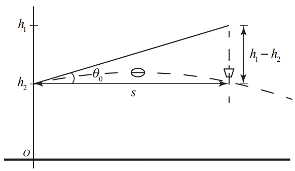
\[\theta_{0}=\tan ^{-1}\left(\left(h_{1}-h_{2}\right) / s\right) \nonumber \]

From the Figure 5.11 we can see that \(\tan \left(\theta_{0}\right)=\left(h_{1}-h_{2}\right) / s\) implies that the second person aims the ball at the initial position of the pail.

Figure 5.11: Geometry of collision

In order to find the time that the ball collides with the pail, we begin by squaring both Equations (5.1.44) and (5.1.43), then utilize the trigonometric identity \(\sin ^{2}\left(\theta_{0}\right)+\cos ^{2}\left(\theta_{0}\right)=1\). Our squared equations become

\[v_{0}^{2} \sin ^{2}\left(\theta_{0}\right) t_{a}^{2}=\left(h_{1}-h_{2}\right)^{2} \nonumber \]

\[v_{0}^{2} \cos ^{2}\left(\theta_{0}\right) t_{a}^{2}=s^{2} \nonumber \]

Adding these equations together and using the identity \(\sin ^{2}\left(\theta_{0}\right)+\cos ^{2}\left(\theta_{0}\right)=1\) and taking square roots yields

\[v_{0} t_{a}=\left(s^{2}+\left(h_{1}-h_{2}\right)^{2}\right)^{1 / 2} \nonumber \]

We can solve Equation (5.1.49) for the time of collision

\[t_{a}=\frac{1}{v_{0}}\left(s^{2}+\left(h_{1}-h_{2}\right)^{2}\right)^{1 / 2} \nonumber \]

We can now use the y -coordinate function of either the ball or the pail at \(t=t_{a}\) to find the height that the ball collides with the pail. Because the pail had no initial y - component of the velocity, it’s easier to use the condition for the pail,

\[y_{1}\left(t_{a}\right)=h_{1}-\frac{g\left(s^{2}+\left(h_{1}-h_{2}\right)^{2}\right)}{2 v_{0}^{2}} \nonumber \]

Comments:

(1) Equations (5.1.49) and (5.1.50) can be arrived at in a very direct way. Suppose we analyze the motion in a reference frame that is accelerating downward with \(\overrightarrow{\mathbf{A}}=-g \hat{\mathbf{j}}\). In that reference frame both the pail and the stone are not accelerating; the pail is at rest and the stone is travelling with speed \(v_{0}\), at an angle \(\theta_{0}\). Therefore in order to hit the stationary pail, the stone must be thrown at the angle given by Equation (5.1.46) and the time that it takes to hit the stone is just given by distance traveled divided by speed, Equation (5.1.50).