22.1: Introduction to Three Dimensional Rotations

Most of the examples and applications we have considered concerned the rotation of rigid bodies about a fixed axis. However, there are many examples of rigid bodies that rotate about an axis that is changing its direction. A turning bicycle wheel, a gyroscope, the earth’s precession about its axis, a spinning top, and a coin rolling on a table are all examples of this type of motion. These motions can be very complex and difficult to analyze. However, for each of these motions we know that if there a non-zero torque about a point \(S\), then the angular momentum about \(S\) must change in time, according to the rotational equation of motion,

\[\vec{\tau}_{S}=\frac{d \overrightarrow{\mathbf{L}}_{S}}{d t} \nonumber \]

We also know that the angular momentum about \(S\) of a rotating body is the sum of the orbital angular momentum about \(S\) and the spin angular momentum about the center of mass.

\[\overrightarrow{\mathbf{L}}_{S}=\overrightarrow{\mathbf{L}}_{S}^{\text {otbial }}+\overrightarrow{\mathbf{L}}_{\mathrm{cm}}^{\text {spin }} \nonumber \]

For fixed axis rotation the spin angular momentum about the center of mass is just

\[\overrightarrow{\mathbf{L}}_{\mathrm{cm}}^{\mathrm{spin}}=I_{\mathrm{cm}} \overrightarrow{\boldsymbol{\omega}}_{\mathrm{cm}} \nonumber \]

where \(\overrightarrow{\boldsymbol{\omega}}_{\mathrm{cm}}\) is the angular velocity about the center of mass and is directed along the fixed axis of rotation.

Angular Velocity for Three Dimensional Rotations

When the axis of rotation is no longer fixed, the angular velocity will no longer point in a fixed direction.

For an object that is rotating with angular coordinates \(\left(\theta_{x}, \theta_{y}, \theta_{z}\right)\) about each respective Cartesian axis, the angular velocity of an object that is rotating about each axis is defined to be

\[\begin{array}{l}
\overrightarrow{\boldsymbol{\omega}}=\frac{d \theta_{x}}{d t} \hat{\mathbf{i}}+\frac{d \theta_{y}}{d t} \hat{\mathbf{j}}+\frac{d \theta_{z}}{d t} \hat{\mathbf{k}} \\
=\omega_{x} \hat{\mathbf{i}}+\omega_{y} \hat{\mathbf{j}}+\omega_{z} \hat{\mathbf{k}}
\end{array} \nonumber \]

This definition is the result of a property of very small (infinitesimal) angular rotations in which the order of rotations does matter. For example, consider an object that undergoes a rotation about the x -axis, \(\overrightarrow{\boldsymbol{\omega}}_{x}=\omega_{x} \hat{\mathbf{i}}\), and then a second rotation about the y -axis, \(\overrightarrow{\boldsymbol{\omega}}_{y}=\omega_{y} \hat{\mathbf{j}}\). Now consider a different sequence of rotations. The object first undergoes a rotation about the y -axis, \(\vec{\omega}_{y}=\omega_{y} \hat{j}\), and then undergoes a second rotation about the x -axis, \(\vec{\omega}_{x}=\omega_{x} \hat{\mathbf{i}}\). In both cases the object will end up in the same position indicated that \(\overrightarrow{\boldsymbol{\omega}}_{x}+\overrightarrow{\boldsymbol{\omega}}_{y}=\overrightarrow{\boldsymbol{\omega}}_{y}+\overrightarrow{\boldsymbol{\omega}}_{x}\) a necessary condition that must be satisfied in order for a physical quantity to be a vector quantity.

Example 22.1 Angular Velocity of a Rolling Bicycle Wheel

A bicycle wheel of mass m and radius R rolls without slipping about the z -axis. An axle of length b passes through its center. The bicycle wheel undergoes two simultaneous rotations. The wheel circles around the z -axis with angular speed Ω and associated angular velocity \(\overrightarrow{\mathbf{\Omega}}=\Omega_{z} \hat{\mathbf{k}}\) (Figure 22.1). Because the wheel is rotating without slipping, it is spinning about its center of mass with angular speed \(\omega_{\mathrm{spin}}\) and associated angular velocity \(\vec{\omega}_{\operatorname{spin}}=-\omega_{\operatorname{spin}} \hat{\mathbf{r}}\)

Figure 22.1 Example 22.1

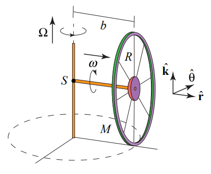
The angular velocity of the wheel is the sum of these two vector contributions

\[\vec{\omega}=\Omega \hat{\mathbf{k}}-\omega_{\mathrm{spin}} \hat{\mathbf{r}} \nonumber \]

Because the wheel is rolling without slipping, \(v_{\mathrm{cm}}=b \Omega=\omega_{\mathrm{spin}} R \text { and so } \omega_{\mathrm{spin}}=b \Omega / R\). The angular velocity is then

\[\overrightarrow{\boldsymbol{\omega}}=\Omega(\hat{\mathbf{k}}-(b / R) \hat{\mathbf{r}}) \nonumber \]

The orbital angular momentum about the point \(S\) where the axle meets the axis of rotation (Figure 22.1), is then

\begin{equation}\overrightarrow{\mathbf{L}}_{S}^{\text {ortital }}=b m v_{\mathrm{cm}} \hat{\mathbf{k}}=m b^{2} \Omega \hat{\mathbf{k}}\end{equation}

The spin angular momentum about the center of mass is more complicated. The wheel is rotating about both the z -axis and the radial axis. Therefore

\[\overrightarrow{\mathbf{L}}_{\mathrm{cm}}^{\mathrm{spin}}=I_{z} \Omega \hat{\mathbf{k}}+I_{r} \omega_{\mathrm{spin}}(-\hat{\mathbf{r}}) \nonumber \]

Therefore the angular momentum about \(S\) is the sum of these two contributions

\[\begin{array}{l}
\overrightarrow{\mathbf{L}}_{S}=m b^{2} \Omega \hat{\mathbf{k}}+I_{z} \Omega \hat{\mathbf{k}}+I_{r} \omega_{\text {spin }}(-\hat{\mathbf{r}}) \\
=\left(m b^{2} \Omega+I_{z} \Omega\right) \hat{\mathbf{k}}-I_{r}(b \Omega / R) \hat{\mathbf{r}}
\end{array} \nonumber \]

Comparing Equations (22.1.6) and (22.1.9), we note that the angular momentum about \(S\) is not proportional to the angular velocity.