25.6: Kepler’s Laws
- Page ID
- 25594
\( \newcommand{\vecs}[1]{\overset { \scriptstyle \rightharpoonup} {\mathbf{#1}} } \)
\( \newcommand{\vecd}[1]{\overset{-\!-\!\rightharpoonup}{\vphantom{a}\smash {#1}}} \)
\( \newcommand{\dsum}{\displaystyle\sum\limits} \)
\( \newcommand{\dint}{\displaystyle\int\limits} \)
\( \newcommand{\dlim}{\displaystyle\lim\limits} \)
\( \newcommand{\id}{\mathrm{id}}\) \( \newcommand{\Span}{\mathrm{span}}\)
( \newcommand{\kernel}{\mathrm{null}\,}\) \( \newcommand{\range}{\mathrm{range}\,}\)
\( \newcommand{\RealPart}{\mathrm{Re}}\) \( \newcommand{\ImaginaryPart}{\mathrm{Im}}\)
\( \newcommand{\Argument}{\mathrm{Arg}}\) \( \newcommand{\norm}[1]{\| #1 \|}\)
\( \newcommand{\inner}[2]{\langle #1, #2 \rangle}\)
\( \newcommand{\Span}{\mathrm{span}}\)
\( \newcommand{\id}{\mathrm{id}}\)
\( \newcommand{\Span}{\mathrm{span}}\)
\( \newcommand{\kernel}{\mathrm{null}\,}\)
\( \newcommand{\range}{\mathrm{range}\,}\)
\( \newcommand{\RealPart}{\mathrm{Re}}\)
\( \newcommand{\ImaginaryPart}{\mathrm{Im}}\)
\( \newcommand{\Argument}{\mathrm{Arg}}\)
\( \newcommand{\norm}[1]{\| #1 \|}\)
\( \newcommand{\inner}[2]{\langle #1, #2 \rangle}\)
\( \newcommand{\Span}{\mathrm{span}}\) \( \newcommand{\AA}{\unicode[.8,0]{x212B}}\)
\( \newcommand{\vectorA}[1]{\vec{#1}} % arrow\)
\( \newcommand{\vectorAt}[1]{\vec{\text{#1}}} % arrow\)
\( \newcommand{\vectorB}[1]{\overset { \scriptstyle \rightharpoonup} {\mathbf{#1}} } \)
\( \newcommand{\vectorC}[1]{\textbf{#1}} \)
\( \newcommand{\vectorD}[1]{\overrightarrow{#1}} \)
\( \newcommand{\vectorDt}[1]{\overrightarrow{\text{#1}}} \)
\( \newcommand{\vectE}[1]{\overset{-\!-\!\rightharpoonup}{\vphantom{a}\smash{\mathbf {#1}}}} \)
\( \newcommand{\vecs}[1]{\overset { \scriptstyle \rightharpoonup} {\mathbf{#1}} } \)
\(\newcommand{\longvect}{\overrightarrow}\)
\( \newcommand{\vecd}[1]{\overset{-\!-\!\rightharpoonup}{\vphantom{a}\smash {#1}}} \)
\(\newcommand{\avec}{\mathbf a}\) \(\newcommand{\bvec}{\mathbf b}\) \(\newcommand{\cvec}{\mathbf c}\) \(\newcommand{\dvec}{\mathbf d}\) \(\newcommand{\dtil}{\widetilde{\mathbf d}}\) \(\newcommand{\evec}{\mathbf e}\) \(\newcommand{\fvec}{\mathbf f}\) \(\newcommand{\nvec}{\mathbf n}\) \(\newcommand{\pvec}{\mathbf p}\) \(\newcommand{\qvec}{\mathbf q}\) \(\newcommand{\svec}{\mathbf s}\) \(\newcommand{\tvec}{\mathbf t}\) \(\newcommand{\uvec}{\mathbf u}\) \(\newcommand{\vvec}{\mathbf v}\) \(\newcommand{\wvec}{\mathbf w}\) \(\newcommand{\xvec}{\mathbf x}\) \(\newcommand{\yvec}{\mathbf y}\) \(\newcommand{\zvec}{\mathbf z}\) \(\newcommand{\rvec}{\mathbf r}\) \(\newcommand{\mvec}{\mathbf m}\) \(\newcommand{\zerovec}{\mathbf 0}\) \(\newcommand{\onevec}{\mathbf 1}\) \(\newcommand{\real}{\mathbb R}\) \(\newcommand{\twovec}[2]{\left[\begin{array}{r}#1 \\ #2 \end{array}\right]}\) \(\newcommand{\ctwovec}[2]{\left[\begin{array}{c}#1 \\ #2 \end{array}\right]}\) \(\newcommand{\threevec}[3]{\left[\begin{array}{r}#1 \\ #2 \\ #3 \end{array}\right]}\) \(\newcommand{\cthreevec}[3]{\left[\begin{array}{c}#1 \\ #2 \\ #3 \end{array}\right]}\) \(\newcommand{\fourvec}[4]{\left[\begin{array}{r}#1 \\ #2 \\ #3 \\ #4 \end{array}\right]}\) \(\newcommand{\cfourvec}[4]{\left[\begin{array}{c}#1 \\ #2 \\ #3 \\ #4 \end{array}\right]}\) \(\newcommand{\fivevec}[5]{\left[\begin{array}{r}#1 \\ #2 \\ #3 \\ #4 \\ #5 \\ \end{array}\right]}\) \(\newcommand{\cfivevec}[5]{\left[\begin{array}{c}#1 \\ #2 \\ #3 \\ #4 \\ #5 \\ \end{array}\right]}\) \(\newcommand{\mattwo}[4]{\left[\begin{array}{rr}#1 \amp #2 \\ #3 \amp #4 \\ \end{array}\right]}\) \(\newcommand{\laspan}[1]{\text{Span}\{#1\}}\) \(\newcommand{\bcal}{\cal B}\) \(\newcommand{\ccal}{\cal C}\) \(\newcommand{\scal}{\cal S}\) \(\newcommand{\wcal}{\cal W}\) \(\newcommand{\ecal}{\cal E}\) \(\newcommand{\coords}[2]{\left\{#1\right\}_{#2}}\) \(\newcommand{\gray}[1]{\color{gray}{#1}}\) \(\newcommand{\lgray}[1]{\color{lightgray}{#1}}\) \(\newcommand{\rank}{\operatorname{rank}}\) \(\newcommand{\row}{\text{Row}}\) \(\newcommand{\col}{\text{Col}}\) \(\renewcommand{\row}{\text{Row}}\) \(\newcommand{\nul}{\text{Nul}}\) \(\newcommand{\var}{\text{Var}}\) \(\newcommand{\corr}{\text{corr}}\) \(\newcommand{\len}[1]{\left|#1\right|}\) \(\newcommand{\bbar}{\overline{\bvec}}\) \(\newcommand{\bhat}{\widehat{\bvec}}\) \(\newcommand{\bperp}{\bvec^\perp}\) \(\newcommand{\xhat}{\widehat{\xvec}}\) \(\newcommand{\vhat}{\widehat{\vvec}}\) \(\newcommand{\uhat}{\widehat{\uvec}}\) \(\newcommand{\what}{\widehat{\wvec}}\) \(\newcommand{\Sighat}{\widehat{\Sigma}}\) \(\newcommand{\lt}{<}\) \(\newcommand{\gt}{>}\) \(\newcommand{\amp}{&}\) \(\definecolor{fillinmathshade}{gray}{0.9}\)Elliptic Orbit Law
I. Each planet moves in an ellipse with the sun at one focus.
When the energy is negative, \(E<0\), and according to Equation (25.3.14),
\[\varepsilon=\left(1+\frac{2 E L^{2}}{\mu\left(G m_{1} m_{2}\right)^{2}}\right)^{\frac{1}{2}} \nonumber \]
and the eccentricity must fall within the range \(0 \leq \varepsilon<1\). These orbits are either circles or ellipses. Note the elliptic orbit law is only valid if we assume that there is only one central force acting. We are ignoring the gravitational interactions due to all the other bodies in the universe, a necessary approximation for our analytic solution.
Equal Area Law
II. The radius vector from the sun to a planet sweeps out equal areas in equal time.
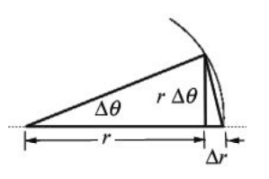
Using analytic geometry in the limit of small Δθ , the sum of the areas of the triangles in Figure 25.9 is given by
\[\Delta A=\frac{1}{2}(r \Delta \theta) r+\frac{(r \Delta \theta)}{2} \Delta r \nonumber \]

The average rate of the change of area, \(\Delta A\), in time, \(\Delta t\), is given by
\[\Delta A=\frac{1}{2} \frac{(r \Delta \theta) r}{\Delta t}+\frac{(r \Delta \theta)}{2} \frac{\Delta r}{\Delta t} \nonumber \]
In the limit as \(\Delta t \rightarrow 0, \Delta \theta \rightarrow 0\), this becomes
\[\frac{d A}{d t}=\frac{1}{2} r^{2} \frac{d \theta}{d t} \label{25.5.4} \]
Recall that according to Equation (25.3.7) (reproduced below as Equation \ref{25.5.5}), the angular momentum is related to the angular velocity \(d \theta / d t\) by
\[\frac{d \theta}{d t}=\frac{L}{\mu r^{2}} \label{25.5.5} \]
and Equation \ref{25.5.4} is then
\[\frac{d A}{d t}=\frac{L}{2 \mu} \label{25.5.6} \]
Because \(L\) and \(\mu\) are constants, the rate of change of area with respect to time is a constant. This is often familiarly referred to by the expression: equal areas are swept out in equal times (see Kepler’s Laws at the beginning of this chapter).
Period Law
III. The period of revolution T of a planet about the sun is related to the semi-major axis a of the ellipse by \(T^{2}=k a^{3}\) where k is the same for all planets.
When Kepler stated his period law for planetary orbits based on observation, he only noted the dependence on the larger mass of the sun. Because the mass of the sun is much greater than the mass of the planets, his observation is an excellent approximation.
In order to demonstrate the third law we begin by rewriting Equation \ref{25.5.6} in the form
\[2 \mu \frac{d A}{d t}=L \label{25.5.7} \]
Equation \ref{25.5.7} can be integrated as
\[\int_{\text {orbit }} 2 \mu d A=\int_{0}^{T} L d t \nonumber \]
where \(T\) is the period of the orbit. For an ellipse,
\[\int_{\text {orbit }}d A=\pi ab \nonumber \]
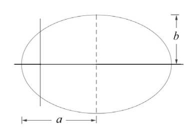
where \(a\) is the semi-major axis and \(b\) is the semi-minor axis (Figure 25.10).

Thus we have
\[T=\frac{2 \mu \pi a b}{L} \label{25.5.10} \]
Squaring Equation \ref{25.5.10} then yields
\[T^{2}=\frac{4 \pi^{2} \mu^{2} a^{2} b^{2}}{L^{2}} \nonumber \]
In Appendix 25B, Equation (25.B.20) gives the angular momentum in terms of the semimajor axis and the eccentricity. Substitution for the angular momentum into Equation (25.5.11) yields
\[T^{2}=\frac{4 \pi^{2} \mu^{2} a^{2} b^{2}}{\mu G m_{1} m_{2} a\left(1-\varepsilon^{2}\right)} \nonumber \]
In Appendix 25B, Equation (25.B.17) gives the semi-minor axis which upon substitution into Equation (25.5.12) yields
\[T^{2}=\frac{4 \pi^{2} \mu^{2} a^{3}}{\mu G m_{1} m_{2}} \nonumber \]
Using Equation (25.2.1) for reduced mass, the square of the period of the orbit is proportional to the semi-major axis cubed,
\[T^{2}=\frac{4 \pi^{2} a^{3}}{G\left(m_{1}+m_{2}\right)} \nonumber \]

