
25.7: Worked Examples
- Page ID
- 25595
\( \newcommand{\vecs}[1]{\overset { \scriptstyle \rightharpoonup} {\mathbf{#1}} } \)
\( \newcommand{\vecd}[1]{\overset{-\!-\!\rightharpoonup}{\vphantom{a}\smash {#1}}} \)
\( \newcommand{\dsum}{\displaystyle\sum\limits} \)
\( \newcommand{\dint}{\displaystyle\int\limits} \)
\( \newcommand{\dlim}{\displaystyle\lim\limits} \)
\( \newcommand{\id}{\mathrm{id}}\) \( \newcommand{\Span}{\mathrm{span}}\)
( \newcommand{\kernel}{\mathrm{null}\,}\) \( \newcommand{\range}{\mathrm{range}\,}\)
\( \newcommand{\RealPart}{\mathrm{Re}}\) \( \newcommand{\ImaginaryPart}{\mathrm{Im}}\)
\( \newcommand{\Argument}{\mathrm{Arg}}\) \( \newcommand{\norm}[1]{\| #1 \|}\)
\( \newcommand{\inner}[2]{\langle #1, #2 \rangle}\)
\( \newcommand{\Span}{\mathrm{span}}\)
\( \newcommand{\id}{\mathrm{id}}\)
\( \newcommand{\Span}{\mathrm{span}}\)
\( \newcommand{\kernel}{\mathrm{null}\,}\)
\( \newcommand{\range}{\mathrm{range}\,}\)
\( \newcommand{\RealPart}{\mathrm{Re}}\)
\( \newcommand{\ImaginaryPart}{\mathrm{Im}}\)
\( \newcommand{\Argument}{\mathrm{Arg}}\)
\( \newcommand{\norm}[1]{\| #1 \|}\)
\( \newcommand{\inner}[2]{\langle #1, #2 \rangle}\)
\( \newcommand{\Span}{\mathrm{span}}\) \( \newcommand{\AA}{\unicode[.8,0]{x212B}}\)
\( \newcommand{\vectorA}[1]{\vec{#1}} % arrow\)
\( \newcommand{\vectorAt}[1]{\vec{\text{#1}}} % arrow\)
\( \newcommand{\vectorB}[1]{\overset { \scriptstyle \rightharpoonup} {\mathbf{#1}} } \)
\( \newcommand{\vectorC}[1]{\textbf{#1}} \)
\( \newcommand{\vectorD}[1]{\overrightarrow{#1}} \)
\( \newcommand{\vectorDt}[1]{\overrightarrow{\text{#1}}} \)
\( \newcommand{\vectE}[1]{\overset{-\!-\!\rightharpoonup}{\vphantom{a}\smash{\mathbf {#1}}}} \)
\( \newcommand{\vecs}[1]{\overset { \scriptstyle \rightharpoonup} {\mathbf{#1}} } \)
\(\newcommand{\longvect}{\overrightarrow}\)
\( \newcommand{\vecd}[1]{\overset{-\!-\!\rightharpoonup}{\vphantom{a}\smash {#1}}} \)
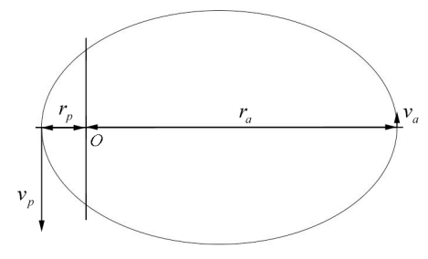
\(\newcommand{\avec}{\mathbf a}\) \(\newcommand{\bvec}{\mathbf b}\) \(\newcommand{\cvec}{\mathbf c}\) \(\newcommand{\dvec}{\mathbf d}\) \(\newcommand{\dtil}{\widetilde{\mathbf d}}\) \(\newcommand{\evec}{\mathbf e}\) \(\newcommand{\fvec}{\mathbf f}\) \(\newcommand{\nvec}{\mathbf n}\) \(\newcommand{\pvec}{\mathbf p}\) \(\newcommand{\qvec}{\mathbf q}\) \(\newcommand{\svec}{\mathbf s}\) \(\newcommand{\tvec}{\mathbf t}\) \(\newcommand{\uvec}{\mathbf u}\) \(\newcommand{\vvec}{\mathbf v}\) \(\newcommand{\wvec}{\mathbf w}\) \(\newcommand{\xvec}{\mathbf x}\) \(\newcommand{\yvec}{\mathbf y}\) \(\newcommand{\zvec}{\mathbf z}\) \(\newcommand{\rvec}{\mathbf r}\) \(\newcommand{\mvec}{\mathbf m}\) \(\newcommand{\zerovec}{\mathbf 0}\) \(\newcommand{\onevec}{\mathbf 1}\) \(\newcommand{\real}{\mathbb R}\) \(\newcommand{\twovec}[2]{\left[\begin{array}{r}#1 \\ #2 \end{array}\right]}\) \(\newcommand{\ctwovec}[2]{\left[\begin{array}{c}#1 \\ #2 \end{array}\right]}\) \(\newcommand{\threevec}[3]{\left[\begin{array}{r}#1 \\ #2 \\ #3 \end{array}\right]}\) \(\newcommand{\cthreevec}[3]{\left[\begin{array}{c}#1 \\ #2 \\ #3 \end{array}\right]}\) \(\newcommand{\fourvec}[4]{\left[\begin{array}{r}#1 \\ #2 \\ #3 \\ #4 \end{array}\right]}\) \(\newcommand{\cfourvec}[4]{\left[\begin{array}{c}#1 \\ #2 \\ #3 \\ #4 \end{array}\right]}\) \(\newcommand{\fivevec}[5]{\left[\begin{array}{r}#1 \\ #2 \\ #3 \\ #4 \\ #5 \\ \end{array}\right]}\) \(\newcommand{\cfivevec}[5]{\left[\begin{array}{c}#1 \\ #2 \\ #3 \\ #4 \\ #5 \\ \end{array}\right]}\) \(\newcommand{\mattwo}[4]{\left[\begin{array}{rr}#1 \amp #2 \\ #3 \amp #4 \\ \end{array}\right]}\) \(\newcommand{\laspan}[1]{\text{Span}\{#1\}}\) \(\newcommand{\bcal}{\cal B}\) \(\newcommand{\ccal}{\cal C}\) \(\newcommand{\scal}{\cal S}\) \(\newcommand{\wcal}{\cal W}\) \(\newcommand{\ecal}{\cal E}\) \(\newcommand{\coords}[2]{\left\{#1\right\}_{#2}}\) \(\newcommand{\gray}[1]{\color{gray}{#1}}\) \(\newcommand{\lgray}[1]{\color{lightgray}{#1}}\) \(\newcommand{\rank}{\operatorname{rank}}\) \(\newcommand{\row}{\text{Row}}\) \(\newcommand{\col}{\text{Col}}\) \(\renewcommand{\row}{\text{Row}}\) \(\newcommand{\nul}{\text{Nul}}\) \(\newcommand{\var}{\text{Var}}\) \(\newcommand{\corr}{\text{corr}}\) \(\newcommand{\len}[1]{\left|#1\right|}\) \(\newcommand{\bbar}{\overline{\bvec}}\) \(\newcommand{\bhat}{\widehat{\bvec}}\) \(\newcommand{\bperp}{\bvec^\perp}\) \(\newcommand{\xhat}{\widehat{\xvec}}\) \(\newcommand{\vhat}{\widehat{\vvec}}\) \(\newcommand{\uhat}{\widehat{\uvec}}\) \(\newcommand{\what}{\widehat{\wvec}}\) \(\newcommand{\Sighat}{\widehat{\Sigma}}\) \(\newcommand{\lt}{<}\) \(\newcommand{\gt}{>}\) \(\newcommand{\amp}{&}\) \(\definecolor{fillinmathshade}{gray}{0.9}\)Example 25.1 Elliptic Orbit
A satellite of mass \(m_{s}\) is in an elliptical orbit around a planet of mass \(m_{p}>>m_{s}\). The planet is located at one focus of the ellipse. The satellite is at the distance \(r_{a}\) when it is furthest from the planet. The distance of closest approach is \(r_{p}\) (Figure 25.11). What is (i) the speed \(v_{p}\) of the satellite when it is closest to the planet and (ii) the speed \(v_{a}\) of the satellite when it is furthest from the planet?
Solution: The angular momentum about the origin is constant and because \(\overrightarrow{\mathbf{r}}_{O, a} \perp \overrightarrow{\mathbf{v}}_{a}\) and \(\overrightarrow{\mathbf{r}}_{O, a} \perp \overrightarrow{\mathbf{v}}_{p}\), the magnitude of the angular momentums satisfies
\[L \equiv L_{O, p}=L_{O_{a}} \nonumber \]
Because \(m_{s}<<m_{p}\) the reduced mass \(\mu \cong m_{s}\) and so the angular momentum condition becomes
\[L=m_{s} r_{p} v_{p}=m r_{s} r v_{a} \nonumber \]
We can solve for \(v_{p}\) in terms of the constants \(G, m_{p}, r_{a} \text { and } r_{p}\) as follows. Choose zero for the gravitational potential energy, \(U(r=\infty)=0\). When the satellite is at the maximum distance from the planet, the mechanical energy is
\[E_{a}=K_{a}+U_{a}=\frac{1}{2} m_{s} v_{a}^{2}-\frac{G m_{s} m_{p}}{r_{a}} \nonumber \]
When the satellite is at closest approach the energy is
\[E_{p}=\frac{1}{2} m_{s} v_{p}^{2}-\frac{G m_{s} m_{p}}{r_{p}} \nonumber \]
When the satellite is at closest approach the energy is
\[E_{p}=\frac{1}{2} m_{s} v_{p}^{2}-\frac{G m_{s} m_{p}}{r_{p}} \nonumber \]
Mechanical energy is constant,
\[E \equiv E_{a}=E_{p} \nonumber \]
therefore
\[E=\frac{1}{2} m_{s} v_{p}^{2}-\frac{G m_{s} m_{p}}{r_{p}}=\frac{1}{2} m_{s} v_{a}^{2}-\frac{G m_{s} m_{p}}{r_{a}} \nonumber \]
From Equation (25.6.2) we know that
\[v_{a}=\left(r_{p} / r_{a}\right) v_{p} \nonumber \]
Substitute Equation (25.6.7) into Equation (25.6.6) and divide through by \(m_{s} / 2\) yields
\[v_{p}^{2}-\frac{2 G m_{p}}{r_{p}}=\frac{r_{p}^{2}}{r_{a}^{2}} v_{p}^{2}-\frac{2 G m_{p}}{r_{a}} \nonumber \]
We can solve this Equation (25.6.8) for \(v_{p}\)
\[\begin{array}{l}
v_{p}^{2}\left(1-\frac{r_{p}^{2}}{r_{a}^{2}}\right)=2 G m_{p}\left(\frac{1}{r_{p}}-\frac{1}{r_{a}}\right) \Rightarrow \\
v_{p}^{2}\left(\frac{r_{a}^{2}-r_{p}^{2}}{r_{a}^{2}}\right)=2 G m_{p}\left(\frac{r_{a}-r_{p}}{r_{p} r_{a}}\right) \Rightarrow \\
v_{p}^{2}\left(\frac{\left(r_{a}-r_{p}\right)\left(r_{a}+r_{p}\right)}{r_{a}^{2}}\right)=2 G m_{p}\left(\frac{r_{a}-r_{p}}{r_{p} r_{a}}\right) \Rightarrow \\
v_{p}=\sqrt{\frac{2 G m_{p} r_{a}}{\left(r_{a}+r_{p}\right) r_{p}}}
\end{array} \nonumber \]
We now use Equation (25.6.7) to determine that
\[v_{a}=\left(r_{p} / r_{a}\right) v_{p}=\sqrt{\frac{2 G m_{p} r_{p}}{\left(r_{a}+r_{p}\right) r_{a}}} \nonumber \]
Example 25.2 The Motion of the Star SO-2 around the Black Hole at the Galactic Center
The UCLA Galactic Center Group, headed by Dr. Andrea Ghez, measured the orbits of many stars within 0.8′′ × 0.8′′ of the galactic center. The orbits of six of those stars are shown in Figure 25.12.
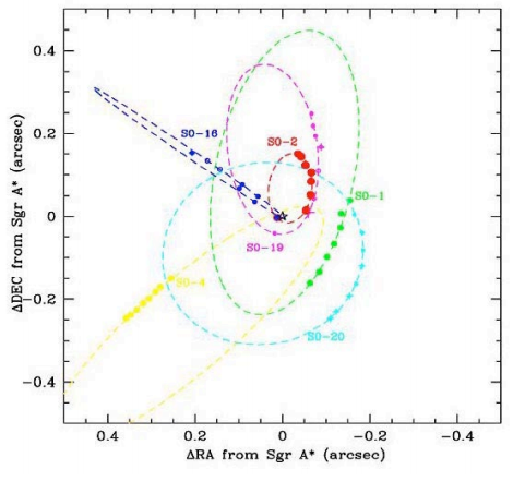
We shall focus on the orbit of the star S0-2 with the following orbit properties given in Table 25.13 . Distances are given in astronomical units, \(1 \mathrm{au}=1.50 \times 10^{11} \mathrm{m}\), which is the mean distance between the earth and the sun.
Table 25.1 Orbital Properties of S0-2
\[\begin{array}{|l|l|l|l|l|l|}
\hline \text { Star } & \begin{array}{l}
\text { Period } \\
\text { (yrs) }
\end{array} & \text { Eccentricity } & \begin{array}{l}
\text { Semi-major } \\
\text { axis } \\
\left(10^{-3} \text {arcsec }\right)
\end{array} & \begin{array}{l}
\text { Periapse } \\
\text { (au) }
\end{array} & \begin{array}{l}
\text { Apoapse } \\
\text { (au) }
\end{array} \\
\hline \text { S0-2 } & \begin{array}{l}
15.2 \\
(0.68 / 0.76)
\end{array} & \begin{array}{l}
0.8763 \\
(0.0063)
\end{array} & 120.7(4.5) & 119.5(3.9) & 1812(73) \\
\hline
\end{array} \nonumber \]
The period of S0-2 satisfies Kepler’s Third Law, given by
\[T^{2}=\frac{4 \pi^{2} a^{3}}{G\left(m_{1}+m_{2}\right)} \nonumber \]
where \(m_{1}\) is the mass of S0-2, \(m_{2}\) is the mass of the black hole, and a is the semi-major axis of the elliptic orbit of S0-2. (a) Determine the mass of the black hole that the star S0- 2 is orbiting. What is the ratio of the mass of the black hole to the solar mass? (b) What is the speed of S0-2 at periapse (distance of closest approach to the center of the galaxy) and apoapse (distance of furthest approach to the center of the galaxy)?
Solution: (a) The semi-major axis is given by
\[a=\frac{r_{p}+r_{a}}{2}=\frac{119.5 \mathrm{au}+1812 \mathrm{au}}{2}=965.8 \mathrm{au} \nonumber \]
In SI units (meters), this is
\[a=965.8 \mathrm{au} \frac{1.50 \times 10^{11} \mathrm{m}}{1 \mathrm{au}}=1.45 \times 10^{14} \mathrm{m} \nonumber \]
The mass \(m_{1}\) of the star S0-2 is much less than the mass of the black hole, and \(m_{2}\) Equation (25.6.11) can be simplified to
\[T^{2}=\frac{4 \pi^{2} a^{3}}{G m_{2}} \nonumber \]
Solving for the mass \(m_{2}\) and inserting the numerical values, yields
\[\begin{aligned}
m_{2} &=\frac{4 \pi^{2} a^{3}}{G T^{2}} \\
&=\frac{\left(4 \pi^{2}\right)\left(1.45 \times 10^{14} \mathrm{m}\right)^{3}}{\left(6.67 \times 10^{-11} \mathrm{N} \cdot \mathrm{m}^{2} \cdot \mathrm{kg}^{-2}\right)\left((15.2 \mathrm{yr})\left(3.16 \times 10^{7} \mathrm{s} \cdot \mathrm{yr}^{-1}\right)\right)^{2}} \\
&=7.79 \times 10^{34} \mathrm{kg}
\end{aligned} \nonumber \]
The ratio of the mass of the black hole to the solar mass is
\[\frac{m_{2}}{m_{\operatorname{sun}}}=\frac{7.79 \times 10^{34} \mathrm{kg}}{1.99 \times 10^{30} \mathrm{kg}}=3.91 \times 10^{6} \nonumber \]
The mass of black hole corresponds to nearly four million solar masses.
(b) We can use our results from Example 25.1 that
\[v_{p}=\sqrt{\frac{2 G m_{2} r_{a}}{\left(r_{a}+r_{p}\right) r_{p}}}=\sqrt{\frac{G m_{2} r_{a}}{a r_{p}}} \nonumber \]
\[v_{a}=\frac{r_{p}}{r_{a}} v_{p}=\sqrt{\frac{2 G m_{2} r_{p}}{\left(r_{a}+r_{p}\right) r_{a}}}=\sqrt{\frac{G m_{2} r_{p}}{a r_{a}}} \nonumber \]
where \(a=\left(r_{a}+r_{b}\right) / 2\) is the semi-major axis. Inserting numerical values,
\[\begin{aligned}
v_{p} &=\sqrt{\frac{G m_{2}}{a} \frac{r_{a}}{r_{p}}} \\
&=\sqrt{\frac{\left(6.67 \times 10^{-11} \mathrm{N} \cdot \mathrm{m}^{2} \cdot \mathrm{kg}^{-2}\right)\left(7.79 \times 10^{34} \mathrm{kg}\right)}{\left(1.45 \times 10^{14} \mathrm{m}\right)}\left(\frac{1812}{119.5}\right)} \\
&=7.38 \times 10^{6} \mathrm{m} \cdot \mathrm{s}^{-1}
\end{aligned} \nonumber \]
The speed \(v_{\mathrm{a}}\) at apoapse is then
\[v_{a}=\frac{r_{p}}{r_{\mathrm{a}}} v_{p}=\left(\frac{1812}{119.5}\right)\left(7.38 \times 10^{6} \mathrm{m} \cdot \mathrm{s}^{-1}\right)=4.87 \times 10^{5} \mathrm{m} \cdot \mathrm{s}^{-1} \nonumber \]
Example 25.3 Central Force Proportional to Distance Cubed
A particle of mass m moves in plane about a central point under an attractive central force of magnitude \(F=b r^{3}\). The magnitude of the angular momentum about the central point is equal to L . (a) Find the effective potential energy and make sketch of effective potential energy as a function of r . (b) Indicate on a sketch of the effective potential the total energy for circular motion. (c) The radius of the particle’s orbit varies between \(r_{0}\) and \(2r_{0}\). Find \(r_{0}\).
Solution: a) The potential energy, taking the zero of potential energy to be at r = 0 , is
\[U(r)=-\int_{0}^{r}\left(-b r^{\prime 3}\right) d r^{\prime}=\frac{b}{4} r^{4} \nonumber \]
The effective potential energy is
\[U_{\mathrm{eff}}(r)=\frac{L^{2}}{2 m r^{2}}+U(r)=\frac{L^{2}}{2 m r^{2}}+\frac{b}{4} r^{4} \nonumber \]
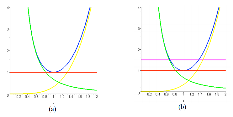
A plot is shown in Figure 25.13a, including the potential (yellow, right-most curve), the term \(L^{2} / 2 m\) (green, left-most curve) and the effective potential (blue, center curve). The horizontal scale is in units of \(r_{0}\) (corresponding to radius of the lowest energy circular orbit) and the vertical scale is in units of the minimum effective potential.
b) The minimum effective potential energy is the horizontal line (red) in Figure 25.13a.
c) We are trying to determine the value of \(r_{0}\) such that \(U_{\mathrm{eff}}\left(r_{0}\right)=U_{\mathrm{eff}}\left(2 r_{0}\right)\). Thus
\[\frac{L^{2}}{m r_{0}^{2}}+\frac{b}{4} r_{0}^{4}=\frac{L^{2}}{m\left(2 r_{0}\right)^{2}}+\frac{b}{4}\left(2 r_{0}\right)^{4} \nonumber \]
Rearranging and combining terms, we can then solve for \(r_{0}\),
\[\begin{array}{c}
\frac{3}{8} \frac{L^{2}}{m} \frac{1}{r_{0}^{2}}=\frac{15}{4} b r_{0}^{4} \\
r_{0}^{6}=\frac{1}{10} \frac{L^{2}}{m b}
\end{array} \nonumber \]
In the plot in Figure 25.13b, if we could move the red line up until it intersects the blue curve at two point whose value of the radius differ by a factor of 2 , those would be the respective values for \(r_{0}\) and \(2r_{0}\). A graph, showing the corresponding energy as the horizontal magenta line, is shown in Figure 25.13b.
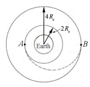
Example 25.4 Transfer Orbit
A space vehicle is in a circular orbit about the earth. The mass of the vehicle is \(m_{\mathrm{s}}=3.00 \times 10^{3} \mathrm{kg}\) and the radius of the orbit is \(2 R_{\mathrm{e}}=1.28 \times 10^{4} \mathrm{km}\). It is desired to transfer the vehicle to a circular orbit of radius \(4 R_{\mathrm{e}}\) (Figure 24.14). The mass of the earth is \(M_{\mathrm{e}}=5.97 \times 10^{24} \mathrm{kg}\). (a) What is the minimum energy expenditure required for the transfer? (b) An efficient way to accomplish the transfer is to use an elliptical orbit from point A on the inner circular orbit to a point B on the outer circular orbit (known as a Hohmann transfer orbit). What changes in speed are required at the points of intersection, A and B?
Solution: (a) The mechanical energy is the sum of the kinetic and potential energies,
\[\begin{aligned}
E &=K+U \\
&=\frac{1}{2} m_{s} v^{2}-G \frac{m_{s} M_{e}}{R_{e}}
\end{aligned} \nonumber \]
For a circular orbit, the orbital speed and orbital radius must be related by Newton’s Second Law,
\[\begin{array}{l}
F_{r}=m a_{r} \\
-G \frac{m_{s} M_{e}}{R_{e}^{2}}=-m_{s} \frac{v^{2}}{R_{e}} \Rightarrow \\
\frac{1}{2} m_{s} v^{2}=\frac{1}{2} G \frac{m_{s} M_{e}}{R_{e}}
\end{array} \nonumber \]
Substituting the last result in (25.6.22) into Equation (25.6.21) yields
\[E=\frac{1}{2} G \frac{m_{s} M_{e}}{R_{e}}-G \frac{m_{s} M_{e}}{R_{e}}=-\frac{1}{2} G \frac{m_{s} M_{e}}{R_{e}}=\frac{1}{2} U\left(R_{e}\right) \nonumber \]
Equation (25.6.23) is one example of what is known as the Virial Theorem, in which the energy is equal to (1/2) the potential energy for the circular orbit. In moving from a circular orbit of radius \(2 R_{\mathrm{e}}\) to a circular orbit of radius \(4 R_{\mathrm{e}}\), the total energy increases, (as the energy becomes less negative). The change in energy is
\[\begin{aligned}
\Delta E &=E\left(r=4 R_{e}\right)-E\left(r=2 R_{e}\right) \\
&=-\frac{1}{2} G \frac{m_{s} M_{e}}{4 R_{e}}-\left(-\frac{1}{2} G \frac{m_{s} M_{e}}{2 R_{e}}\right) \\
&=\frac{G m_{s} M_{e}}{8 R_{e}}
\end{aligned} \nonumber \]
Inserting the numerical values,
\[\begin{aligned}
\Delta E &=\frac{1}{8} G \frac{m_{s} M_{e}}{R_{e}}=\frac{1}{4} G \frac{m_{s} M_{e}}{2 R_{e}} \\
&=\frac{1}{4}\left(6.67 \times 10^{-11} \mathrm{m}^{3} \cdot \mathrm{kg}^{-1} \cdot \mathrm{s}^{-2}\right) \frac{\left(3.00 \times 10^{3} \mathrm{kg}\right)\left(5.97 \times 10^{24} \mathrm{kg}\right)}{\left(1.28 \times 10^{4} \mathrm{km}\right)} \\
&=2.3 \times 10^{10} \mathrm{J}
\end{aligned} \nonumber \]
b) The satellite must increase its speed at point A in order to move to the larger orbit radius and increase its speed again at point B to stay in the new circular orbit. Denote the satellite speed at point A while in the circular orbit as \(v_{A, i}\) and after the speed increase (a “rocket burn”) as \(v_{A, f}\) Similarly, denote the satellite’s speed when it first reaches point B as \(v_{B, i}\) Once the satellite reaches point B , it then needs to increase its speed in order to continue in a circular orbit. Denote the speed of the satellite in the circular orbit at point B by \(\mathcal{v}_{B, f}\). The speeds \(v_{A, i}\) and \(v_{B, f}\) are given by Equation (25.6.22). While the satellite is moving from point A to point B in the elliptic orbit (that is, during the transfer, after the first burn and before the second), both mechanical energy and angular momentum are conserved. Conservation of energy relates the speeds and radii by
\[\frac{1}{2} m_{s}\left(v_{A, f}\right)^{2}-G \frac{m_{s} m_{e}}{2 R_{e}}=\frac{1}{2} m_{s}\left(v_{B, t}\right)^{2}-G \frac{m_{s} m_{e}}{4 R_{e}} \nonumber \]
Conservation of angular momentum relates the speeds and radii by
\[m_{s} v_{A, f}\left(2 R_{e}\right)=m_{s} v_{B, i}\left(4 R_{e}\right) \Rightarrow v_{A, f}=2 v_{B, i} \nonumber \]
Substitution of Equation (25.6.27) into Equation (25.6.26) yields, after minor algebra,
\[v_{A, f}=\sqrt{\frac{2 G M_{e}}{3}}, \quad v_{B, i}=\sqrt{\frac{1}{6} \frac{G M_{e}}{R_{e}}} \nonumber \]
We can now use Equation (25.6.22) to determine that
\[v_{A, i}=\sqrt{\frac{1}{2} \frac{G M_{e}}{R_{e}}}, \quad v_{B, f}=\sqrt{\frac{1}{4} \frac{G M_{e}}{R_{e}}} \nonumber \]
Thus the change in speeds at the respective points is given by
\[\begin{array}{l}
\Delta v_{A}=v_{A, f}-v_{A, i}=(\sqrt{\frac{2}{3}}-\sqrt{\frac{1}{2}}) \sqrt{\frac{G M_{e}}{R_{e}}} \\
\Delta v_{B}=v_{B, f}-v_{B, i}=(\sqrt{\frac{1}{4}}-\sqrt{\frac{1}{6}}) \sqrt{\frac{G M_{e}}{R_{e}}}
\end{array} \nonumber \]
Substitution of numerical values gives
\[\Delta v_{A}=8.6 \times 10^{2} \mathrm{m} \cdot \mathrm{s}^{-2}, \quad \Delta v_{B}=7.2 \times 10^{2} \mathrm{m} \cdot \mathrm{s}^{-2} \nonumber \]