Physics LibreTexts

25.9: Appendix 25B Properties of an Elliptical Orbit

  • Page ID
    25597
  • \( \newcommand{\vecs}[1]{\overset { \scriptstyle \rightharpoonup} {\mathbf{#1}} } \) \( \newcommand{\vecd}[1]{\overset{-\!-\!\rightharpoonup}{\vphantom{a}\smash {#1}}} \)\(\newcommand{\id}{\mathrm{id}}\) \( \newcommand{\Span}{\mathrm{span}}\) \( \newcommand{\kernel}{\mathrm{null}\,}\) \( \newcommand{\range}{\mathrm{range}\,}\) \( \newcommand{\RealPart}{\mathrm{Re}}\) \( \newcommand{\ImaginaryPart}{\mathrm{Im}}\) \( \newcommand{\Argument}{\mathrm{Arg}}\) \( \newcommand{\norm}[1]{\| #1 \|}\) \( \newcommand{\inner}[2]{\langle #1, #2 \rangle}\) \( \newcommand{\Span}{\mathrm{span}}\) \(\newcommand{\id}{\mathrm{id}}\) \( \newcommand{\Span}{\mathrm{span}}\) \( \newcommand{\kernel}{\mathrm{null}\,}\) \( \newcommand{\range}{\mathrm{range}\,}\) \( \newcommand{\RealPart}{\mathrm{Re}}\) \( \newcommand{\ImaginaryPart}{\mathrm{Im}}\) \( \newcommand{\Argument}{\mathrm{Arg}}\) \( \newcommand{\norm}[1]{\| #1 \|}\) \( \newcommand{\inner}[2]{\langle #1, #2 \rangle}\) \( \newcommand{\Span}{\mathrm{span}}\)\(\newcommand{\AA}{\unicode[.8,0]{x212B}}\)

    25B.1 Coordinate System for the Elliptic Orbit

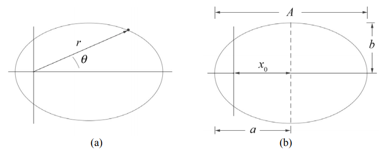
    We now consider the special case of an elliptical orbit. Choose coordinates with the central point located at one focal point and coordinates \((r, \theta)\) for the position of the single body (Figure 25B.1a). In Figure 25B.1b, let a denote the semi-major axis, b denote the semi-minor axis and \(x_{0}\) denote the distance from the center of the ellipse to the origin of our coordinate system.

    clipboard_e267defbf92b2c420caedc7eb563ae943.png
    Figure 25B.1 (a) Coordinate system for elliptic orbit, (b) semi-major axis

    25B.2 The Semi-major Axis

    Recall the orbit equation, Eq, (25.A.9), describes r(θ),

    \[r(\theta)=\frac{r_{0}}{1-\varepsilon \cos \theta} \nonumber \]

    The major axis A = 2a is given by

    \[A=2 a=r_{a}+r_{p} \nonumber \]

    where the distance of furthest approach \(r_{a}\) occurs when \(\theta=0\), hence

    \[r_{a}=r(\theta=0)=\frac{r_{0}}{1-\varepsilon} \nonumber \]

    and the distance of nearest approach \(\boldsymbol{r}_{p}\) occurs when \(\theta=\pi\), hence

    \[r_{p}=r(\theta=\pi)=\frac{r_{0}}{1+\varepsilon} \nonumber \]

    Figure 25B.2 shows the distances of nearest and furthest approach.

    clipboard_e9bc26e842351e7677918548fd853e46f.png
    Figure 25B.2 Furthest and nearest approach

    We can now determine the semi-major axis

    \[a=\frac{1}{2}\left(\frac{r_{0}}{1-\varepsilon}+\frac{r_{0}}{1+\varepsilon}\right)=\frac{r_{0}}{1-\varepsilon^{2}} \nonumber \]

    The semilatus rectum \(r_{0}\) can be re-expressed in terms of the semi-major axis and the eccentricity,

    \[r_{0}=a\left(1-\varepsilon^{2}\right) \nonumber \]

    We can now express the distance of nearest approach, Equation (25.B.4), in terms of the semi-major axis and the eccentricity,

    \[r_{p}=\frac{r_{0}}{1+\varepsilon}=\frac{a\left(1-\varepsilon^{2}\right)}{1+\varepsilon}=a(1-\varepsilon) \nonumber \]

    In a similar fashion the distance of furthest approach is

    \[r_{a}=\frac{r_{0}}{1-\varepsilon}=\frac{a\left(1-\varepsilon^{2}\right)}{1-\varepsilon}=a(1+\varepsilon) \nonumber \]

    25B.2.3 The Location \(x_{0}\) of the Center of the Ellipse

    From Figure 25B.3a, the distance from a focus point to the center of the ellipse is

    \[x_{0}=a-r_{p} \nonumber \]

    clipboard_e599e398f20d266c4f0e654a6707a1374.png
    Figure 25B.3 Location of the center of the ellipse and semi-minor axis.

    Using Equation (25.B.7) for \(r_{p}\), we have that

    \[x_{0}=a-a(1-\varepsilon)=\varepsilon a \nonumber \]

    25B.2.4 The Semi-minor Axis

    From Figure 25B.3b, the semi-minor axis can be expressed as

    \[b=\sqrt{\left(r_{b}^{2}-x_{0}^{2}\right)} \nonumber \]

    where

    \[r_{b}=\frac{r_{0}}{1-\varepsilon \cos \theta_{b}} \nonumber \]

    We can rewrite Equation (25.B.12) as

    \[r_{b}-r_{b} \varepsilon \cos \theta_{b}=r_{0} \nonumber \]

    The horizontal projection of \(r_{b}\) is given by (Figure 25B.2b),

    \[x_{0}=r_{b} \cos \theta_{b} \nonumber \]

    which upon substitution into Equation (25.B.13) yields

    \[r_{b}=r_{0}+\varepsilon x_{0} \nonumber \]

    Substituting Equation (25.B.10) for \(x_{0}\) and Equation (25.B.6) for \(r_{0}\) into Equation (25.B.15) yields

    \[r_{b}=a\left(1-\varepsilon^{2}\right)+a \varepsilon^{2}=a \nonumber \]

    The fact that \(r_{b}=a\) is a well-known property of an ellipse reflected in the geometric construction, that the sum of the distances from the two foci to any point on the ellipse is a constant. We can now determine the semi-minor axis b by substituting Equation (25.B.16) into Equation (25.B.11) yielding

    \[b=\sqrt{\left(r_{b}^{2}-x_{0}^{2}\right)}=\sqrt{a^{2}-\varepsilon^{2} a^{2}}=a \sqrt{1-\varepsilon^{2}} \nonumber \]

    25B.2.5 Constants of the Motion for Elliptic Motion

    We shall now express the parameters a , b and \(x_{0}\) in terms of the constants of the motion L , E , \(\mu\), \(m_{1}\) and \(m_{2}\). Using our results for \(r_{0}\) and \(\varepsilon\) from Equations (25.3.13) and (25.3.14) we have for the semi-major axis

    \[\begin{aligned}
    a &=\frac{L^{2}}{\mu G m_{1} m_{2}} \frac{1}{\left(1-\left(1+2 E L^{2} / \mu\left(G m_{1} m_{2}\right)^{2}\right)\right)} \\
    &=-\frac{G m_{1} m_{2}}{2 E}
    \end{aligned} \nonumber \]

    The energy is then determined by the semi-major axis,

    \[E=-\frac{G m_{1} m_{2}}{2 a} \nonumber \]

    The angular momentum is related to the semilatus rectum \(r_{0}\) by Equation (25.3.13). Using Equation (25.B.6) for \(r_{0}\), we can express the angular momentum (25.B.4) in terms of the semi-major axis and the eccentricity,

    \[L=\sqrt{\mu G m_{1} m_{2} r_{0}}=\sqrt{\mu G m_{1} m_{2} a\left(1-\varepsilon^{2}\right)} \nonumber \]

    Note that

    \[\sqrt{\left(1-\varepsilon^{2}\right)}=\frac{L}{\sqrt{\mu G m_{1} m_{2} a}} \nonumber \]

    Thus, from Equations (25.3.14), (25.B.10), and (25.B.18), the distance from the center of the ellipse to the focal point is

    \[x_{0}=\varepsilon a=-\frac{G m_{1} m_{2}}{2 E} \sqrt{\left(1+2 E L^{2} / \mu\left(G m_{1} m_{2}\right)^{2}\right)} \nonumber \]

    a result we will return to later. We can substitute Equation (25.B.21) for \(\sqrt{1-\varepsilon^{2}}\) into Equation (25.B.17), and determine that the semi-minor axis is

    \[b=\sqrt{a L^{2} / \mu G m_{1} m_{2}} \nonumber \]

    We can now substitute Equation (25.B.18) for a into Equation (25.B.23), yielding

    \[b=\sqrt{a L^{2} / \mu G m_{1} m_{2}}=L \sqrt{-\frac{G m_{1} m_{2}}{2 E} / \mu G m_{1} m_{2}}=L \sqrt{-\frac{1}{2 \mu E}} \nonumber \]

    25B.2.6 Speeds at Nearest and Furthest Approaches

    At nearest approach, the velocity vector is tangent to the orbit (Figure 25B.4), so the magnitude of the angular momentum is

    \[L=\mu r_{p} v_{p} \nonumber \]

    and the speed at nearest approach is

    \[v_{p}=L / \mu r_{p} \nonumber \]

    clipboard_edd0b0318217e413bce4ed04fd354ff4a.png
    Figure 25B.4 Speeds at nearest and furthest approach

    Using Equation (25.B.20) for the angular momentum and Equation (25.B.7) for r p , Equation (25.B.26) becomes

    \[v_{p}=\frac{L}{\mu r_{p}}=\frac{\sqrt{\mu G m_{1} m_{2}\left(1-\varepsilon^{2}\right)}}{\mu a(1-\varepsilon)}=\sqrt{\frac{G m_{1} m_{2}\left(1-\varepsilon^{2}\right)}{\mu a(1-\varepsilon)^{2}}}=\sqrt{\frac{G m_{1} m_{2}(1+\varepsilon)}{\mu a(1-\varepsilon)}} \nonumber \]

    A similar calculation show that the speed \(v_{a}\) at furthest approach,

    \[v_{a}=\frac{L}{\mu r_{a}}=\frac{\sqrt{\mu G m_{1} m_{2}\left(1-\varepsilon^{2}\right)}}{\mu a(1+\varepsilon)}=\sqrt{\frac{G m_{1} m_{2} 1-\varepsilon^{2}}{\mu a(1+\varepsilon)^{2}}}=\sqrt{\frac{G m_{1} m_{2}(1-\varepsilon)}{\mu a(1+\varepsilon)}} \nonumber \]


    This page titled 25.9: Appendix 25B Properties of an Elliptical Orbit is shared under a not declared license and was authored, remixed, and/or curated by Peter Dourmashkin (MIT OpenCourseWare) via source content that was edited to the style and standards of the LibreTexts platform; a detailed edit history is available upon request.