4.2: Inertia Tensor

Since the dynamics of each point of a rigid body is strongly constrained by the conditions \(r_{k k}\) ’ = const, this is one of the most important fields of application of the Lagrangian formalism discussed in Chapter 2. For using this approach, the first thing we need to calculate is the kinetic energy of the body in an inertial reference frame. Since it is just the sum of the kinetic energies (1.19) of all its points, we can use Eq. (10) to write: \({ }^{4}\) \[T \equiv \sum \frac{m}{2} \mathbf{v}^{2}=\sum \frac{m}{2}\left(\mathbf{v}_{0}+\boldsymbol{\omega} \times \mathbf{r}\right)^{2}=\sum \frac{m}{2} v_{0}^{2}+\sum m \mathbf{v}_{0} \cdot(\boldsymbol{\omega} \times \mathbf{r})+\sum \frac{m}{2}(\boldsymbol{\omega} \times \mathbf{r})^{2} .\] Let us apply to the right-hand side of Eq. (11) two general vector analysis formulas listed in the Math Appendix: the so-called operand rotation rule MA Eq. (7.6) to the second term, and MA Eq. (7.7b) to the third term. The result is \[T=\sum \frac{m}{2} v_{0}^{2}+\sum m \mathbf{r} \cdot\left(\mathbf{v}_{0} \times \boldsymbol{\omega}\right)+\sum \frac{m}{2}\left[\omega^{2} r^{2}-(\boldsymbol{\omega} \cdot \mathbf{r})^{2}\right] .\] This expression may be further simplified by making a specific choice of the point 0 (from that the radius vectors \(\mathbf{r}\) of all particles are measured), namely by using for this point the center of mass of the body. As was already mentioned in Sec. \(3.4\) for the 2-point case, the radius vector \(\mathbf{R}\) of this point is defined as \[M \mathbf{R} \equiv \sum m \mathbf{r}, \quad M \equiv \sum m,\] where \(M\) is the total mass of the body. In the reference frame centered as this point, \(\mathbf{R}=0\), so that the second sum in Eq. (12) vanishes, and the kinetic energy is a sum of just two terms: \[T=T_{\text {tran }}+T_{\text {rot }}, \quad T_{\text {tran }} \equiv \frac{M}{2} V^{2}, \quad T_{\text {rot }} \equiv \sum \frac{m}{2}\left[\omega^{2} r^{2}-(\boldsymbol{\omega} \cdot \mathbf{r})^{2}\right]\] where \(\mathbf{V} \equiv d \mathbf{R} / d t\) is the center-of-mass velocity in our inertial reference frame, and all particle positions \(\mathbf{r}\) are measured in the center-of-mass frame. Since the angular velocity vector \(\omega\) is common for all points of a rigid body, it is more convenient to rewrite the rotational energy in a form in that the summation over the components of this vector is clearly separated from the summation over the points of the body: \[T_{\mathrm{rot}}=\frac{1}{2} \sum_{j, j^{\prime}=1}^{3} I_{j j^{\prime}} \omega_{j} \omega_{j^{\prime}},\] where the \(3 \times 3\) matrix with elements \[I_{j j^{\prime}} \equiv \sum m\left(r^{2} \delta_{j j^{\prime}}-r_{j} r_{j^{\prime}}\right)\] is called the inertia tensor of the body. \({ }^{5}\)

Actually, the term "tensor" for this matrix has to be justified, because in physics this term implies a certain reference-frame-independent notion, whose elements have to obey certain rules at the transfer between reference frames. To show that the matrix (16) indeed deserves its title, let us calculate another key quantity, the total angular momentum \(\mathbf{L}\) of the same body. \({ }^{6}\) Summing up the angular momenta of each particle, defined by Eq. (1.31), and then using Eq. (10) again, in our inertial reference frame we get \[\mathbf{L} \equiv \sum \mathbf{r} \times \mathbf{p}=\sum m \mathbf{r} \times \mathbf{v}=\sum m \mathbf{r} \times\left(\mathbf{v}_{0}+\boldsymbol{\omega} \times \mathbf{r}\right) \equiv \sum m \mathbf{r} \times \mathbf{v}_{0}+\sum m \mathbf{r} \times(\boldsymbol{\omega} \times \mathbf{r}) .\] We see that the momentum may be represented as a sum of two terms. The first one, \[\mathbf{L}_{0} \equiv \sum m \mathbf{r} \times \mathbf{v}_{0}=M \mathbf{R} \times \mathbf{v}_{0},\] describes the possible rotation of the center of mass around the inertial frame’s origin. This term evidently vanishes if the moving reference frame’s origin 0 is positioned at the center of mass (where \(\mathbf{R}\) \(=0)\). In this case, we are left with only the second term, which describes a pure rotation of the body about its center of mass: \[\mathbf{L}=\mathbf{L}_{\mathrm{rot}} \equiv \sum m \mathbf{r} \times(\boldsymbol{\omega} \times \mathbf{r})\] Using one more vector algebra formula, the "bac minis cab" rule, \({ }^{7}\) we may rewrite this expression as \[\mathbf{L}=\sum m\left[\boldsymbol{\omega} r^{2}-\mathbf{r}(\mathbf{r} \cdot \boldsymbol{\omega})\right] .\] Let us spell out an arbitrary Cartesian component of this vector: \[L_{j}=\sum m\left[\omega_{j} r^{2}-r_{j} \sum_{j^{\prime}=1}^{3} r_{j^{\prime}} \omega_{j^{\prime}}\right] \equiv \sum m \sum_{j^{\prime}=1}^{3} \omega_{j^{\prime}}\left(r^{2} \delta_{i j^{\prime}}-r_{j} r_{j^{\prime}}\right) .\] By changing the summation order and comparing the result with Eq. (16), the angular momentum may be conveniently expressed via the same matrix elements \(I_{i j}\) ’ as the rotational kinetic energy: \[L_{j}=\sum_{j^{\prime}=1}^{3} I_{j j^{\prime}} \omega_{j^{\prime}} .\] Since \(\mathbf{L}\) and \(\omega\) are both legitimate vectors (meaning that they describe physical vectors independent of the reference frame choice), their connection, the matrix of elements \(I_{i j}\), is a legitimate tensor. This fact, and the symmetry of the tensor \(\left(I_{i j^{\prime}}=I_{j^{\prime} j}\right)\), which is evident from its definition (16), allow the tensor to be further simplified. In particular, mathematics tells us that by a certain choice of the axes’ orientations, any symmetric tensor may be reduced to a diagonal form \[I_{j j^{\prime}}=I_{j} \delta_{j j^{\prime}},\] where in our case \[I_{j}=\sum m\left(r^{2}-r_{j}^{2}\right)=\sum m\left(r_{j^{\prime}}^{2}+r_{j^{\prime}}^{2}\right) \equiv \sum m \rho_{j}^{2},\] being the distance of the particle from the \(j^{\text {th }}\) axis, i.e. the length of the perpendicular dropped from the point to that axis. The axes of such a special coordinate system are called the principal axes, while the diagonal elements \(I_{j}\) given by Eq. (24), the principal moments of inertia of the body. In such a special reference frame, Eqs. (15) and (22) are reduced to very simple forms: \[\begin{gathered} T_{\mathrm{rot}}=\sum_{j=1}^{3} \frac{I_{j}}{2} \omega_{j}^{2}, \\ L_{j}=I_{j} \omega_{j} . \end{gathered}\] Both these results remind the corresponding relations for the translational motion, \(T_{\text {tran }}=M V^{2} / 2\) and \(\mathbf{P}=\) \(M \mathbf{V}\), with the angular velocity \(\omega\) replacing the linear velocity \(\mathbf{V}\), and the tensor of inertia playing the role of scalar mass \(M\). However, let me emphasize that even in the specially selected reference frame, with axes pointing in principal directions, the analogy is incomplete, and rotation is generally more complex than translation, because the measures of inertia, \(I_{j}\), are generally different for each principal axis.

Let me illustrate this fact on a simple but instructive system of three similar massive particles fixed in the vertices of an equilateral triangle (Figure 3).

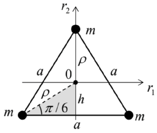Figure 4.3. Principal moments of inertia: a simple case study.

Due to the symmetry of the configuration, one of the principal axes has to pass through the center of mass 0 and be normal to the plane of the triangle. For the corresponding principal moment of inertia, Eq. (24) readily yields \(I_{3}=3 m \rho^{2}\). If we want to express the result in terms of the triangle side \(a\), we may notice that due to the system’s symmetry, the angle marked in Figure 3 equals \(\pi / 6\), and from the shaded right triangle, \(a / 2=\rho \cos (\pi / 6) \equiv \rho \sqrt{3} / 2\), giving \(\rho=a / \sqrt{3}\), so that, finally, \(I_{3}=m a^{2}\).

Let me use this simple case to illustrate the following general axis shift theorem, which may be rather useful - especially for more complex systems. For that, let us relate the inertia tensor components \(I_{j j^{\prime}}\) and \(I_{j j^{\prime}}^{\prime}\), calculated in two reference frames - one with the origin in the center of mass 0 , and another one \(\left(0^{\prime}\right)\) displaced by a certain vector \(\mathbf{d}\) (Figure 4a), so that for an arbitrary point, \(\mathbf{r}^{\prime}=\mathbf{r}+\mathbf{d}\). Plugging this relation into Eq. (16), we get \[\begin{aligned} I^{\prime}{ }_{j j^{\prime}}^{\prime} &=\sum m\left[(\mathbf{r}+\mathbf{d})^{2} \delta_{j j^{\prime}}-\left(r_{j}+d_{j}\right)\left(r_{j^{\prime}}+d_{j^{\prime}}\right)\right] \\ &=\sum m\left[\left(r^{2}+2 \mathbf{r} \cdot \mathbf{d}+d^{2}\right) \delta_{j j^{\prime}}-\left(r_{j} r_{j^{\prime}}+r_{j} d_{j^{\prime}}+r_{j^{\prime}} d_{j}+d_{j} d_{j^{\prime}}\right)\right] . \end{aligned}\] Since in the center-of-mass frame, all sums \(\sum m r_{j}\) equal zero, we may use Eq. (16) to finally obtain \[I_{j j^{\prime}}^{\prime}=I_{j j^{\prime}}+M\left(\delta_{j j^{\prime}} d^{2}-d_{j} d_{j^{\prime}}\right) .\] In particular, this equation shows that if the shift vector \(\mathbf{d}\) is perpendicular to one (say, \(j^{\text {th }}\) ) of the principal axes (Figure \(4 \mathrm{~b}\) ), i.e. \(d_{j}=0\), then Eq. (28) is reduced to a very simple formula:

Principal axis’

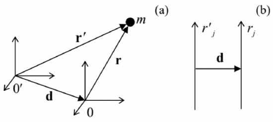Figure 4.4. (a) A general reference frame’s shift from the center of mass, and (b) a shift perpendicular to one of the principal axes.

Now returning to the system shown in Figure 3, let us perform such a shift to the new ("primed") axis passing through the location of one of the particles, still perpendicular to the particles’ plane. Then the contribution of that particular mass to the primed moment of inertia vanishes, and \(I_{3}^{\prime}=2 \mathrm{ma}^{2}\). Now, returning to the center of mass and applying Eq. (29), we get \(I_{3}=I_{3}-M \rho^{2}=2 m a^{2}-(3 m)(a / \sqrt{3})^{2}=m a^{2}\), i.e. the same result as above.

The symmetry situation inside the triangle’s plane is somewhat less evident, so let us start with calculating the moments of inertia for the axes shown vertical and horizontal in Figure 3. From Eq. (24) we readily get: \[I_{1}=2 m h^{2}+m \rho^{2}=m\left[2\left(\frac{a}{2 \sqrt{3}}\right)^{2}+\left(\frac{a}{\sqrt{3}}\right)^{2}\right]=\frac{m a^{2}}{2}, \quad I_{2}=2 m\left(\frac{a}{2}\right)^{2}=\frac{m a^{2}}{2},\] where \(h\) is the distance from the center of mass and any side of the triangle: \(h=\rho \sin (\pi / 6)=\rho / 2=\) \(a / 2 \sqrt{3}\). We see that \(I_{1}=I_{2}\), and mathematics tells us that in this case any in-plane axis (passing through the center-of-mass 0 ) may be considered as principal, and has the same moment of inertia. A rigid body Symmetric
top: with this property, \(I_{1}=I_{2} \neq I_{3}\), is called the symmetric top. (The last direction is called the main principal with this property, \(I_{1}=I_{2} \neq I_{3}\), is called the symmetric top. (The last direction is called the main principal axis of the system.)

Despite the symmetric top’s name, the situation may be even more symmetric in the so-called spherical tops, i.e. highly symmetric systems whose principal moments of inertia are all equal, \[I_{1}=I_{2}=I_{3} \equiv I,\] Mathematics says that in this case, the moment of inertia for rotation about any axis (but still passing through the center of mass) is equal to the same \(I\). Hence Eqs. (25) and (26) are further simplified for any direction of the vector \(\omega\) : \[T_{\text {rot }}=\frac{I}{2} \omega^{2}, \quad \mathbf{L}=I \omega\] thus making the analogy of rotation and translation complete. (As will be discussed in the next section, this analogy is also complete if the rotation axis is fixed by external constraints.)

Evident examples of a spherical top are a uniform sphere and a uniform spherical shell; a less obvious example is a uniform cube - with masses either concentrated in vertices, or uniformly spread over the faces, or uniformly distributed over the volume. Again, in this case any axis passing through the center of mass is principal and has the same principal moment of inertia. For a sphere, this is natural; for a cube, rather surprising - but may be confirmed by a direct calculation.

---

\({ }^{4}\) Actually, all symbols for particle masses, coordinates, and velocities should carry the particle’s index, over which the summation is carried out. However, in this section, for the notation simplicity, this index is just implied.

\({ }^{5}\) While the \(\mathrm{ABCs}\) of the rotational dynamics were developed by Leonhard Euler in 1765 , an introduction of the inertia tensor’s formalism had to wait very long - until the invention of the tensor analysis by Tullio Levi-Civita and Gregorio Ricci-Curbastro in 1900 - soon popularized by its use in Einstein’s theory of general relativity.

\({ }^{6}\) Hopefully, there is very little chance of confusing the angular momentum \(\mathbf{L}\) (a vector) and its Cartesian components \(L_{j}\) (scalars with an index) on one hand, and the Lagrangian function \(L\) (a scalar without an index) on the other hand.

\({ }^{7}\) See, e.g., MA Eq. (7.5).