
4.3: Fixed-axis Rotation
- Page ID
- 34762

\( \newcommand{\vecs}[1]{\overset { \scriptstyle \rightharpoonup} {\mathbf{#1}} } \)
\( \newcommand{\vecd}[1]{\overset{-\!-\!\rightharpoonup}{\vphantom{a}\smash {#1}}} \)
\( \newcommand{\dsum}{\displaystyle\sum\limits} \)
\( \newcommand{\dint}{\displaystyle\int\limits} \)
\( \newcommand{\dlim}{\displaystyle\lim\limits} \)
\( \newcommand{\id}{\mathrm{id}}\) \( \newcommand{\Span}{\mathrm{span}}\)
( \newcommand{\kernel}{\mathrm{null}\,}\) \( \newcommand{\range}{\mathrm{range}\,}\)
\( \newcommand{\RealPart}{\mathrm{Re}}\) \( \newcommand{\ImaginaryPart}{\mathrm{Im}}\)
\( \newcommand{\Argument}{\mathrm{Arg}}\) \( \newcommand{\norm}[1]{\| #1 \|}\)
\( \newcommand{\inner}[2]{\langle #1, #2 \rangle}\)
\( \newcommand{\Span}{\mathrm{span}}\)
\( \newcommand{\id}{\mathrm{id}}\)
\( \newcommand{\Span}{\mathrm{span}}\)
\( \newcommand{\kernel}{\mathrm{null}\,}\)
\( \newcommand{\range}{\mathrm{range}\,}\)
\( \newcommand{\RealPart}{\mathrm{Re}}\)
\( \newcommand{\ImaginaryPart}{\mathrm{Im}}\)
\( \newcommand{\Argument}{\mathrm{Arg}}\)
\( \newcommand{\norm}[1]{\| #1 \|}\)
\( \newcommand{\inner}[2]{\langle #1, #2 \rangle}\)
\( \newcommand{\Span}{\mathrm{span}}\) \( \newcommand{\AA}{\unicode[.8,0]{x212B}}\)
\( \newcommand{\vectorA}[1]{\vec{#1}} % arrow\)
\( \newcommand{\vectorAt}[1]{\vec{\text{#1}}} % arrow\)
\( \newcommand{\vectorB}[1]{\overset { \scriptstyle \rightharpoonup} {\mathbf{#1}} } \)
\( \newcommand{\vectorC}[1]{\textbf{#1}} \)
\( \newcommand{\vectorD}[1]{\overrightarrow{#1}} \)
\( \newcommand{\vectorDt}[1]{\overrightarrow{\text{#1}}} \)
\( \newcommand{\vectE}[1]{\overset{-\!-\!\rightharpoonup}{\vphantom{a}\smash{\mathbf {#1}}}} \)
\( \newcommand{\vecs}[1]{\overset { \scriptstyle \rightharpoonup} {\mathbf{#1}} } \)
\(\newcommand{\longvect}{\overrightarrow}\)
\( \newcommand{\vecd}[1]{\overset{-\!-\!\rightharpoonup}{\vphantom{a}\smash {#1}}} \)
\(\newcommand{\avec}{\mathbf a}\) \(\newcommand{\bvec}{\mathbf b}\) \(\newcommand{\cvec}{\mathbf c}\) \(\newcommand{\dvec}{\mathbf d}\) \(\newcommand{\dtil}{\widetilde{\mathbf d}}\) \(\newcommand{\evec}{\mathbf e}\) \(\newcommand{\fvec}{\mathbf f}\) \(\newcommand{\nvec}{\mathbf n}\) \(\newcommand{\pvec}{\mathbf p}\) \(\newcommand{\qvec}{\mathbf q}\) \(\newcommand{\svec}{\mathbf s}\) \(\newcommand{\tvec}{\mathbf t}\) \(\newcommand{\uvec}{\mathbf u}\) \(\newcommand{\vvec}{\mathbf v}\) \(\newcommand{\wvec}{\mathbf w}\) \(\newcommand{\xvec}{\mathbf x}\) \(\newcommand{\yvec}{\mathbf y}\) \(\newcommand{\zvec}{\mathbf z}\) \(\newcommand{\rvec}{\mathbf r}\) \(\newcommand{\mvec}{\mathbf m}\) \(\newcommand{\zerovec}{\mathbf 0}\) \(\newcommand{\onevec}{\mathbf 1}\) \(\newcommand{\real}{\mathbb R}\) \(\newcommand{\twovec}[2]{\left[\begin{array}{r}#1 \\ #2 \end{array}\right]}\) \(\newcommand{\ctwovec}[2]{\left[\begin{array}{c}#1 \\ #2 \end{array}\right]}\) \(\newcommand{\threevec}[3]{\left[\begin{array}{r}#1 \\ #2 \\ #3 \end{array}\right]}\) \(\newcommand{\cthreevec}[3]{\left[\begin{array}{c}#1 \\ #2 \\ #3 \end{array}\right]}\) \(\newcommand{\fourvec}[4]{\left[\begin{array}{r}#1 \\ #2 \\ #3 \\ #4 \end{array}\right]}\) \(\newcommand{\cfourvec}[4]{\left[\begin{array}{c}#1 \\ #2 \\ #3 \\ #4 \end{array}\right]}\) \(\newcommand{\fivevec}[5]{\left[\begin{array}{r}#1 \\ #2 \\ #3 \\ #4 \\ #5 \\ \end{array}\right]}\) \(\newcommand{\cfivevec}[5]{\left[\begin{array}{c}#1 \\ #2 \\ #3 \\ #4 \\ #5 \\ \end{array}\right]}\) \(\newcommand{\mattwo}[4]{\left[\begin{array}{rr}#1 \amp #2 \\ #3 \amp #4 \\ \end{array}\right]}\) \(\newcommand{\laspan}[1]{\text{Span}\{#1\}}\) \(\newcommand{\bcal}{\cal B}\) \(\newcommand{\ccal}{\cal C}\) \(\newcommand{\scal}{\cal S}\) \(\newcommand{\wcal}{\cal W}\) \(\newcommand{\ecal}{\cal E}\) \(\newcommand{\coords}[2]{\left\{#1\right\}_{#2}}\) \(\newcommand{\gray}[1]{\color{gray}{#1}}\) \(\newcommand{\lgray}[1]{\color{lightgray}{#1}}\) \(\newcommand{\rank}{\operatorname{rank}}\) \(\newcommand{\row}{\text{Row}}\) \(\newcommand{\col}{\text{Col}}\) \(\renewcommand{\row}{\text{Row}}\) \(\newcommand{\nul}{\text{Nul}}\) \(\newcommand{\var}{\text{Var}}\) \(\newcommand{\corr}{\text{corr}}\) \(\newcommand{\len}[1]{\left|#1\right|}\) \(\newcommand{\bbar}{\overline{\bvec}}\) \(\newcommand{\bhat}{\widehat{\bvec}}\) \(\newcommand{\bperp}{\bvec^\perp}\) \(\newcommand{\xhat}{\widehat{\xvec}}\) \(\newcommand{\vhat}{\widehat{\vvec}}\) \(\newcommand{\uhat}{\widehat{\uvec}}\) \(\newcommand{\what}{\widehat{\wvec}}\) \(\newcommand{\Sighat}{\widehat{\Sigma}}\) \(\newcommand{\lt}{<}\) \(\newcommand{\gt}{>}\) \(\newcommand{\amp}{&}\) \(\definecolor{fillinmathshade}{gray}{0.9}\)Now we are well equipped for a discussion of rigid body’s rotational dynamics. The general equation of this dynamics is given by Eq. (1.38), which is valid for dynamics of any system of particles - either rigidly connected or not: \[\dot{\mathbf{L}}=\boldsymbol{\tau},\] where \(\tau\) is the net torque of external forces. Let us start exploring this equation from the simplest case when the axis of rotation, i.e. the direction of vector \(\omega\), is fixed by some external constraints. Directing the \(z\)-axis along this vector, we have \(\omega_{x}=\omega_{y}=0\). According to Eq. (22), in this case, the \(z\)-component of the angular momentum, \[L_{z}=I_{z z} \omega_{z},\] where \(I_{z z}\), though not necessarily one of the principal moments of inertia, still may be calculated using Eq. (24): \[I_{z z}=\sum m \rho_{z}^{2}=\sum m\left(x^{2}+y^{2}\right),\] with \(\rho_{z}\) being the distance of each particle from the rotation axis \(z\). According to Eq. (15), in this case the rotational kinetic energy is just \[T_{\text {rot }}=\frac{I_{z z}}{2} \omega_{z}^{2} .\] Moreover, it is straightforward to show that if the rotation axis is fixed, Eqs. (34)-(36) are valid even if the axis does not pass through the center of mass - provided that the distances \(\rho_{z}\) are now measured from that axis. (The proof is left for the reader’s exercise.)
As a result, we may not care about other components of the vector \(\mathbf{L},{ }^{8}\) and use just one component of Eq. (33), \[\dot{L}_{z}=\tau_{z},\] because it, when combined with Eq. (34), completely determines the dynamics of rotation: \[I_{z z} \dot{\omega}_{z}=\tau_{z}, \quad \text { i.e. } I_{z z} \ddot{\theta}_{z}=\tau_{z},\] where \(\theta_{z}\) is the angle of rotation about the axis, so that \(\omega_{z}=\dot{\theta}\). The scalar relations (34), (36) and (38), describing rotation about a fixed axis, are completely similar to the corresponding formulas of 1D motion of a single particle, with \(\omega_{z}\) corresponding to the usual ("linear") velocity, the angular momentum component \(L_{z}\) - to the linear momentum, and \(I_{z}\)-to particle’s mass.
The resulting motion about the axis is also frequently similar to that of a single particle. As a simple example, let us consider what is called the physical pendulum (Figure 5) - a rigid body free to rotate about a fixed horizontal axis that does not pass through the center of mass 0 , in a uniform gravity field \(\mathbf{g}\).
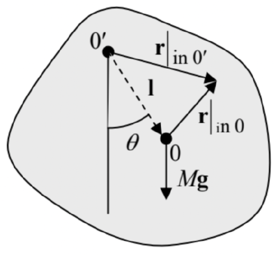 Figure 4.5. Physical pendulum: a body with a fixed (horizontal) rotation axis 0' that does not pass through the center of mass 0 . (The plane of drawing is normal to the axis.)
Let us drop the perpendicular from point 0 to the rotation axis, and call the oppositely directed vector \(\mathbf{l}\) - see the dashed arrow in Figure 5. Then the torque (relative to the rotation axis 0 ’) of the forces keeping the axis fixed is zero, and the only contribution to the net torque is due to gravity alone: \[\left.\left.\boldsymbol{\tau}\right|_{\text {in } 0^{\prime}} \equiv \sum \mathbf{r}\right|_{\text {in } 0^{\prime}} \times \mathbf{F}=\sum\left(\mathbf{l}+\left.\mathbf{r}\right|_{\text {in } 0}\right) \times m \mathbf{g}=\sum m(\mathbf{l} \times \mathbf{g})+\left.\sum m \mathbf{r}\right|_{\text {in } 0} \times \mathbf{g}=M \mathbf{l} \times \mathbf{g} .\] (The last step used the facts that point 0 is the center of mass, so that the second term in the right-hand side equals zero, and that the vectors \(\mathbf{l}\) and \(\mathbf{g}\) are the same for all particles of the body.)
This result shows that the torque is directed along the rotation axis, and its (only) component \(\tau_{z}\) is equal to \(-M g l \sin \theta\), where \(\theta\) is the angle between the vectors \(\mathbf{l}\) and \(\mathbf{g}\), i.e. the angular deviation of the pendulum from the position of equilibrium - see Figure 5 again. As a result, Eq. (38) takes the form, \[I^{\prime} \ddot{\theta}=-M g l \sin \theta,\] where \(I^{\prime}\) is the moment of inertia for rotation about the axis 0 ’ rather than about the center of mass. This equation is identical to Eq. (1.18) for the point-mass (sometimes called "mathematical") pendulum, with the small-oscillation frequency \[\Omega=\left(\frac{M g l}{I^{\prime}}\right)^{1 / 2}\] As a sanity check, in the simplest case when the linear size of the body is much smaller than the suspension length \(l\), Eq. (35) yields \(I^{\prime}=M l^{2}\), and Eq. (41) reduces to the well-familiar formula \(\Omega=\) \((g / l)^{1 / 2}\) for the point-mass pendulum.
Now let us discuss the situations when a rigid body not only rotates but also moves as a whole. As we already know from our introductory chapter, the total linear momentum of the body, \[\mathbf{P} \equiv \sum m \mathbf{v}=\sum m \dot{\mathbf{r}}=\frac{d}{d t} \sum m \mathbf{r}\] satisfies the \(2^{\text {nd }}\) Newton law in the form (1.30). Using the definition (13) of the center of mass, the momentum may be represented as \[\begin{gathered} \mathbf{P}=M \dot{\mathbf{R}}=M \mathbf{V}, \\ M \dot{\mathbf{V}}=\mathbf{F}, \end{gathered}\] where \(\mathbf{F}\) is the vector sum of all external forces. This equation shows that the center of mass of the body moves exactly like a point particle of mass \(M\), under the effect of the net force \(\mathbf{F}\). In many cases, this fact makes the translational dynamics of a rigid body absolutely similar to that of a point particle.
The situation becomes more complex if some of the forces contributing to the vector sum \(\mathbf{F}\) depend on the rotation of the same body, i.e. if its rotational and translational motions are coupled. Analysis of such coupled motion is rather straightforward if the direction of the rotation axis does not change in time, and hence Eqs. (35)-(36) are still valid. Possibly the simplest example is a round cylinder (say, a wheel) rolling on a surface without slippage (Figure 6). Here the no-slippage condition may be represented as the requirement of the net velocity of the particular wheel’s point A that touches the surface to equal zero - in the reference frame connected to the surface. For the simplest case of plane surface (Figure 6a), this condition may be spelled out using Eq. (10), giving the following relation between the angular velocity \(\omega\) of the wheel and the linear velocity \(V\) of its center:
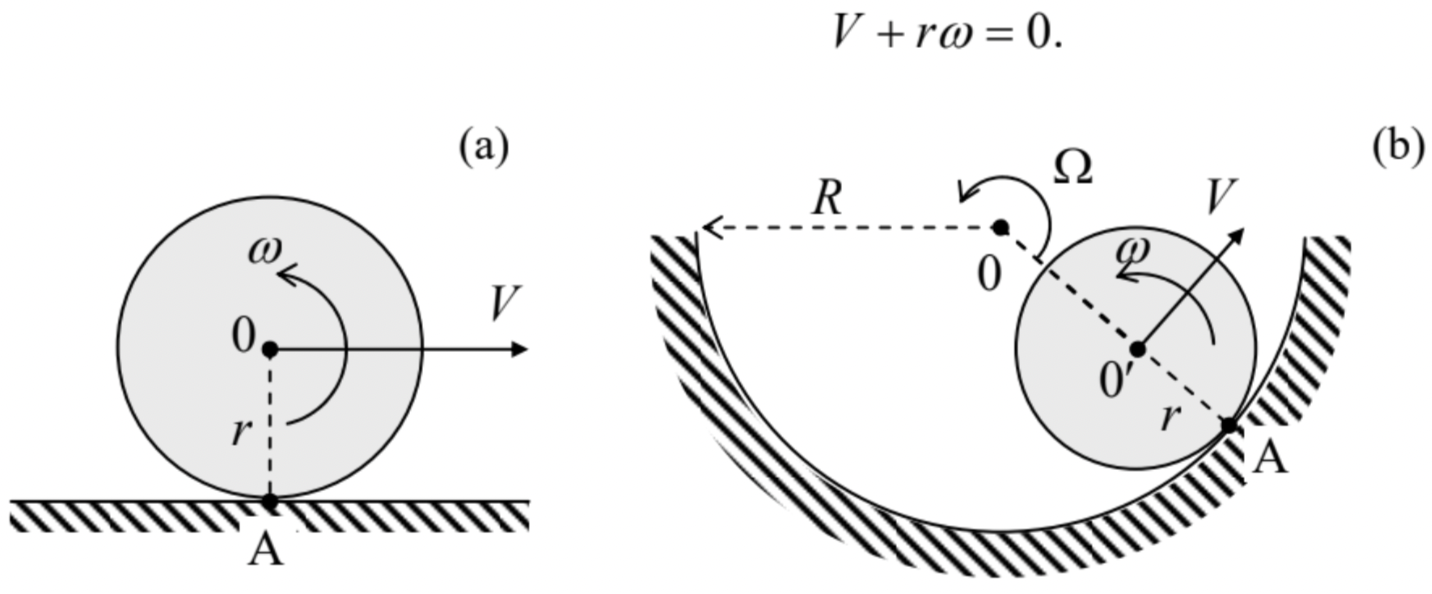 Figure 4.6. Round cylinder rolling over (a) a plane surface and (b) a concave surface.
Such kinematic relations are essentially holonomic constraints, which reduce the number of degrees of freedom of the system. For example, without the no-slippage condition (45), the wheel on a plane surface has to be considered as a system with two degrees of freedom, making its total kinetic energy (14) a function of two independent generalized velocities, say \(V\) and \(\omega\) : \[T=T_{\text {tran }}+T_{\text {rot }}=\frac{M}{2} V^{2}+\frac{I}{2} \omega^{2} .\] Using Eq. (45) we may eliminate, for example, the linear velocity and reduce Eq. (46) to \[T=\frac{M}{2}(\omega r)^{2}+\frac{I}{2} \omega^{2} \equiv \frac{I_{\mathrm{ef}}}{2} \omega^{2}, \quad \text { where } I_{\mathrm{ef}} \equiv I+M r^{2} .\] This result may be interpreted as the kinetic energy of pure rotation of the wheel about the instantaneous rotation axis A, with \(I_{\text {ef }}\) being the moment of inertia about that axis, satisfying Eq. (29).
Kinematic relations are not always as simple as Eq. (45). For example, if a wheel is rolling on a concave surface (Figure 6b), we need to relate the angular velocities of the wheel’s rotation about its axis 0 ’ (say, \(\omega\) ) and that (say, \(\Omega\) ) of its axis’ rotation about the center 0 of curvature of the surface. A popular error here is to write \(\Omega=-(r / R) \omega\) [WRONG!]. A prudent way to derive the correct relation is to note that Eq. (45) holds for this situation as well, and on the other hand, the same linear velocity of the wheel’s center may be expressed as \(V=(R-r) \Omega\). Combining these formulas, we get the correct relation \[\Omega=-\frac{r}{R-r} \omega .\] Another famous example of the relation between the translational and rotational motion is given by the "sliding ladder" problem (Figure 7). Let us analyze it for the simplest case of negligible friction, and the ladder’s thickness small in comparison with its length \(l\).
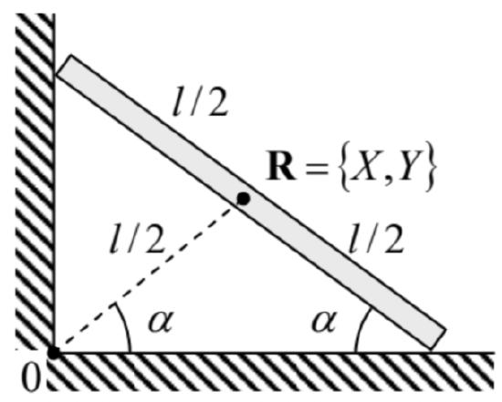 Figure 4.7. The sliding ladder problem.
To use the Lagrangian formalism, we may write the kinetic energy of the ladder as the sum (14) of its translational and rotational parts: \[T=\frac{M}{2}\left(\dot{X}^{2}+\dot{Y}^{2}\right)+\frac{I}{2} \dot{\alpha}^{2},\] where \(X\) and \(Y\) are the Cartesian coordinates of its center of mass in an inertial reference frame, and \(I\) is the moment of inertia for rotation about the \(z\)-axis passing through the center of mass. (For the uniformly distributed mass, an elementary integration of Eq. (35) yields \(I=M l^{2} / 12\) ). In the reference frame with the center in the corner 0 , both \(X\) and \(Y\) may be simply expressed via the angle \(\alpha\) : \[X=\frac{l}{2} \cos \alpha, \quad Y=\frac{l}{2} \sin \alpha .\] (The easiest way to obtain these relations is to notice that the dashed line in Figure 7 has length \(l / 2\), and the same slope \(\alpha\) as the ladder.) Plugging these expressions into Eq. (49), we get \[T=\frac{I_{\mathrm{ef}}}{2} \dot{\alpha}^{2}, \quad I_{\mathrm{ef}} \equiv I+M\left(\frac{l}{2}\right)^{2}=\frac{1}{3} M l^{2} .\] Since the potential energy of the ladder in the gravity field may be also expressed via the same angle, \[U=M g Y=M g \frac{l}{2} \sin \alpha,\] \(\alpha\) may be conveniently used as the (only) generalized coordinate of the system. Even without writing the Lagrange equation of motion for that coordinate, we may notice that since the Lagrangian function \(L\) \(\equiv T-U\) does not depend on time explicitly, and the kinetic energy (51) is a quadratic-homogeneous function of the generalized velocity \(\dot{\alpha}\), the full mechanical energy, \[E \equiv T+U=\frac{I_{\mathrm{ef}}}{2} \dot{\alpha}^{2}+M g \frac{l}{2} \sin \alpha=\frac{M g l}{2}\left(\frac{l \dot{\alpha}^{2}}{3 g}+\sin \alpha\right),\] is conserved, giving us the first integral of motion. Moreover, Eq. (53) shows that the system’s energy (and hence dynamics) is identical to that of a physical pendulum with an unstable fixed point \(\alpha_{1}=\pi / 2\), a stable fixed point at \(\alpha_{2}=-\pi / 2\), and frequency \[\Omega=\left(\frac{3 g}{2 l}\right)^{1 / 2}\] of small oscillations near the latter point. (Of course, this fixed point cannot be reached in the simple geometry shown in Figure 7, where the ladder’s fall on the floor would change its equations of motion. Moreover, even before that, the left end of the ladder may detach from the wall. The analysis of this issue is left for the reader’s exercise.)
\({ }^{8}\) Note that according to Eq. (22), other Cartesian components of the angular momentum, \(L_{x}\) and \(L_{y}\), may be different from zero, and may even evolve in time. The corresponding torques \(\tau_{x}\) and \(\tau_{y}\), which obey Eq. (33), are automatically provided by the external forces that keep the rotation axis fixed.