5.6: Fixed Point Classification

The reduced equations (79) give us a good pretext for a brief discussion of an important general topic of dynamics: fixed points of a system described by two time-independent, first-order differential equations with time-independent coefficients. \({ }^{29}\) After their linearization near a fixed point, the equations for deviations can always be expressed in the form similar to Eq. (79): \[\begin{aligned} &\dot{\tilde{q}}_{1}=M_{11} \widetilde{q}_{1}+M_{12} \widetilde{q}_{2}, \\ &\dot{\widetilde{q}}_{2}=M_{21} \widetilde{q}_{1}+M_{22} \widetilde{q}_{2}, \end{aligned}\] where \(M_{i j^{\prime}}\) (with \(j, j^{\prime}=1,2\) ) are some real scalars, which may be viewed as the elements of a \(2 \times 2\) matrix M. Looking for an exponential solution of the type (80), \[\widetilde{q}_{1}=c_{1} e^{\lambda t}, \quad \widetilde{q}_{2}=c_{2} e^{\lambda t},\] we get a general system of two linear equations for the distribution coefficients \(c_{1,2}\) : \[\begin{aligned} &\left(M_{11}-\lambda\right) c_{1}+M_{12} c_{2}=0, \\ &M_{21} c_{1}+\left(M_{22}-\lambda\right) c_{2}=0 . \end{aligned}\] These equations are consistent if \[\left|\begin{array}{cc} M_{11}-\lambda & M_{12} \\ M_{21} & M_{22}-\lambda \end{array}\right|=0\] giving us a quadratic characteristic equation: \[\lambda^{2}-\lambda\left(M_{11}+M_{22}\right)+\left(M_{11} M_{22}-M_{12} M_{21}\right)=0 .\] Its solution, \({ }^{30}\) \[\lambda_{\pm}=\frac{1}{2}\left(M_{11}+M_{22}\right) \pm \frac{1}{2}\left[\left(M_{11}-M_{22}\right)^{2}+4 M_{12} M_{21}\right]^{1 / 2},\] shows that the following situations are possible:

A. The expression under the square root, \(\left(M_{11}-M_{22}\right)^{2}+4 M_{12} M_{21}\), is positive. In this case, both characteristic exponents \(\lambda_{\pm}\)are real, and we can distinguish three sub-cases:

(i) Both \(\lambda_{+}\)and \(\lambda_{-}\)are negative. As Eqs. (88) show, in this case the deviations \(\widetilde{q}\) tend to zero at \(t \rightarrow \infty\), i.e. fixed point is stable. Because of generally different magnitudes of the exponents \(\lambda_{\pm}\), the process represented on the phase plane \(\left[\widetilde{q}_{1}, \widetilde{q}_{2}\right]\) (see Figure 8a, with the solid arrows, for an example) may be seen as consisting of two stages: first, a faster (with the rate \(\left|\lambda_{-}\right|>\left|\lambda_{+}\right|\)) relaxation to a linear asymptote, \({ }^{31}\) and then a slower decline, with the rate \(\left|\lambda_{+}\right|\), along this line, i.e. at a virtually fixed ratio of the variables. Such a fixed point is called the stable node.

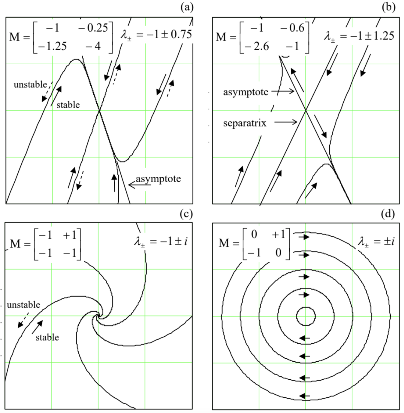
Figure 5.8. Typical trajectories on the phase plane \(\left[\widetilde{q}_{1}, \widetilde{q}_{2}\right]\) near fixed points of different types: (a) node, (b) saddle, (c) focus, and (d) center. The particular elements of the matrix M, used in the first three panels, correspond to Eqs. (81) for the parametric excitation, with \(\xi=\delta\) and three different values of the ratio \(\mu \omega / 4 \delta\) : (a) \(1.25\), (b) \(1.6\), and (c) 0 .

(ii) Both \(\lambda_{+}\)and \(\lambda_{\text {are positive. This case of an unstable node differs from the previous }}\) one only by the direction of motion along the phase plane trajectories - see the dashed arrows in Figure 8a. Here the variable ratio is also approaching a constant soon, now the one corresponding to \(\lambda_{+}>\lambda\).

(iii) Finally, in the case of a saddle \(\left(\lambda_{+}>0, \lambda_{-}<0\right)\), the system’s dynamics is different (Figure 8b): after the rate- \(\lambda_{-} \mid\)relaxation to an asymptote, the perturbation starts to grow, with the rate \(\lambda_{+}\), along one of two opposite directions. (The direction is determined on which side of another straight line, called the separatrix, the system has been initially.) So the saddle \({ }^{32}\) is an unstable fixed point.

B. The expression under the square root in Eq. (92), \(\left(M_{11}-M_{22}\right)^{2}+4 M_{12} M_{21}\), is negative. In this case, the square root is imaginary, making the real parts of both roots equal, \(\operatorname{Re} \lambda_{\pm}=\left(M_{11}+M_{22}\right) / 2\), and their imaginary parts equal but opposite. As a result, here there can be just two types of fixed points:

(i) Stable focus, at \(\left(M_{11}+M_{22}\right)<0\). The phase plane trajectories are spirals going to the origin (i.e. toward the fixed point) - see Figure \(8 \mathrm{c}\) with the solid arrow.

(ii) Unstable focus, taking place at \(\left(M_{11}+M_{22}\right)>0\), differs from the stable one only by the direction of motion along the phase trajectories - see the dashed arrow in the same Figure 8c.

C. Frequently, the border case, \(M_{11}+M_{22}=0\), corresponding to the orbital ("indifferent") stability already discussed in Sec. 3.2, is also distinguished, and the corresponding fixed point is referred to as the center (Figure 8d). Considering centers as a separate category makes sense because such fixed points are typical for Hamiltonian systems, whose first integral of motion may be frequently represented as the distance of the phase point from a fixed point. For example, introducing new variables \(\widetilde{q}_{1} \equiv \tilde{q}, \tilde{q}_{2} \equiv m \dot{\tilde{q}}_{1}\), we may rewrite Eq. (3.12) of a harmonic oscillator without dissipation (again, with indices "ef" dropped for brevity), as a system of two first-order differential equations: \[\dot{\tilde{q}}_{1}=\frac{1}{m} \widetilde{q}_{2}, \quad \dot{\widetilde{q}}_{2}=-\kappa \tilde{q}_{1},\] i.e. as a particular case of Eq. (87), with \(M_{11}=M_{22}=0\), and \(M_{12} M_{21}=-\kappa / m \equiv-\omega_{0}^{2}<0\), and hence \(\left(M_{11}-\right.\) \(\left.M_{22}\right)^{2}+4 M_{12} M_{21}=-4 \omega_{0}^{2}<0\), and \(M_{11}+M_{22}=0\). On the symmetrized phase plane \(\left[\widetilde{q}_{1}, \widetilde{q}_{2} / Z\right]\), where the parameter \(Z \equiv(\kappa m)^{1 / 2} \equiv m \omega_{0}\) is the oscillator’s impedance, the sinusoidal oscillations of amplitude \(A\) are represented by a circle of radius \(A\) about the center-type fixed point \(A=0\). In the case when \(\widetilde{q}_{1} \equiv \widetilde{q}\) is the linear coordinate \(q\) of an actual mechanical oscillator, so that \(\widetilde{q}_{2} \equiv m \dot{\widetilde{q}}_{1}\) is its linear momentum \(p=m \dot{q}\), such a circular trajectory corresponds to the conservation of the oscillator’s energy \[E \equiv T+U \equiv \frac{p^{2}}{2 m}+\frac{\kappa q^{2}}{2} \equiv \frac{\kappa}{2}\left[\widetilde{q}_{1}^{2}+\left(\frac{\widetilde{q}_{2}}{Z}\right)^{2}\right]=\frac{\kappa A^{2}}{2}=\mathrm{const}\] This is a convenient moment for a brief discussion of the so-called Poincaré (or "slow-variable", or "stroboscopic") plane. \({ }^{33}\) From the point of view of the basic Eq. (41), the sinusoidal oscillations \(q(t)\) \(=A \cos (\omega t-\varphi)\), described by a circular trajectory on the actual (symmetrized) phase plane, correspond to a fixed point \(\{A, \varphi\}\), which may be conveniently represented by a stationary geometric point on the plane with these polar coordinates - see Figure 9a. (As follows from Eq. (4), the Cartesian coordinates of the point on that plane are just the variables \(u \equiv A \cos \varphi\) and \(v \equiv A \cos \varphi\) that were used, in particular, in the last section.) The quasi-sinusoidal process (41), with slowly changing \(A\) and \(\varphi\), may be represented by a slow motion of that point on this Poincaré plane.

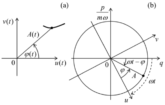Figure 5.9. (a) Representation of a sinusoidal oscillation (point) and a slow transient process (line) on the Poincaré plane, and (b) the relation between the "fast" phase plane and the "slow" (Poincaré) plane.

Figure \(9 \mathrm{~b}\) shows a convenient way to visualize the relation between the actual phase plane of an oscillator, with the "fast" symmetrized coordinates \(q\) and \(p / m \omega\), and the Poincaré plane with the "slow" coordinates \(u\) and \(v\) : the latter plane rotates relative to the former one, about the origin, clockwise, with the angular velocity \(\omega .{ }^{34}\) Another, "stroboscopic" way to generate the Poincare plane pattern is to have a fast glance at the "real" phase plane just once during the oscillation period \(T=2 \pi / \omega\).

In many cases, the representation on the Poincaré plane is more convenient than that on the "real" phase plane. In particular, we have already seen that the reduced equations for such important phenomena as the phase locking and the parametric oscillations, whose original differential equations include time explicitly, are time-independent - cf., e.g., \((75)\) and \((79)\) describing the latter effect. This simplification brings the equations into the category considered earlier in this section, and enables an easy classification of their fixed points, which may shed additional light on their dynamic properties.

In particular, Figure 10 shows the classification of the only (trivial) fixed point \(A_{1}=0\) on the Poincaré plane of the parametric oscillator, which follows from Eq. (83). As the parameter modulation depth \(\mu\) is increased, the type of this fixed point changes from a stable focus (pertinent to a simple oscillator with damping) to a stable node and then to a saddle describing the parametric excitation. In the last case, the two directions of the perturbation growth, so prominently featured in Figure \(8 \mathrm{~b}\), correspond to the two possible values of the oscillation phase \(\varphi\), with the phase choice determined by initial conditions.

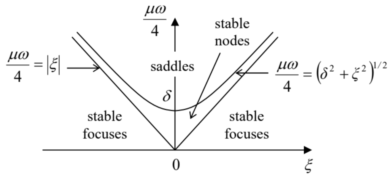Fig. 5.10. Types of the trivial fixed point of a parametric oscillator.

This double degeneracy of the parametric oscillation’s phase could already be noticed from Eqs. (77), because they are evidently invariant with respect to the replacement \(\varphi \rightarrow \varphi+\pi\). Moreover, the degeneracy is not an artifact of the van der Pol approximation, because the initial equation (75) is already invariant with respect to the corresponding replacement \(q(t) \rightarrow q(t-\pi / \omega)\). This invariance means that all other characteristics (including the amplitude) of the parametric oscillations excited with either of the two phases are exactly similar. At the dawn of the computer age (in the late 1950s and early \(1960 \mathrm{~s}\) ), there were substantial attempts, especially in Japan, to use this property for storage and processing digital information coded in the phase-binary form. Though these attempts have not survived the competition with simpler approaches based on voltage-binary coding, some current trends in the development of prospective reversible and quantum computers may be traced back to that idea.

---

\({ }^{29}\) Autonomous systems described by a single, second-order homogeneous differential equation, say \(F(q, \dot{q}, \ddot{q})=0\), also belong to this class, because we may always treat the generalized velocity \(\dot{q} \equiv v\) as a new variable, and use this definition as one first-order differential equation, while the initial equation, in the form \(F(q, v, \dot{v})=0\), as the second first-order equation.

\({ }^{30}\) In the language of linear algebra, \(\lambda_{\pm}\)are the eigenvalues, and the corresponding sets of the distribution coefficients \(\left[c_{1}, c_{2}\right]_{\pm}\)are the eigenvectors of the matrix \(\mathrm{M}\) with elements \(M_{j j}\) ’.

\({ }^{31}\) The asymptote direction may be found by plugging the value \(\lambda_{+}\)back into Eq. (89) and finding the corresponding ratio \(c_{1} / c_{2}\). Note that the separation of the system’s evolution into the two stages is conditional, being most vivid in the case of a large difference between the exponents \(\lambda_{+}\)and \(\lambda\).

\({ }^{32}\) The term "saddle" is due to the fact that in this case, the system’s dynamics is qualitatively similar to that of a heavily damped motion in a 2D potential \(U\left(\widetilde{q}_{1}, \widetilde{q}_{2}\right)\) having the shape of a horse saddle (or a mountain pass).

\({ }^{33}\) Named after Jules Henri Poincaré \((1854-1912)\), who is credited, among many other achievements in physics and mathematics, for his contributions to special relativity (see, e.g., EM Chapter 9), and the basic idea of unstable trajectories responsible for the deterministic chaos - to be discussed in Chapter 9 of this course.

\({ }^{34}\) This notion of phase plane rotation is the origin of the term "Rotating Wave Approximation", mentioned above. (The word "wave" is an artifact of this method’s wide application in classical and quantum optics.)