
5.7: Numerical Approaches
- Page ID
- 58630
\( \newcommand{\vecs}[1]{\overset { \scriptstyle \rightharpoonup} {\mathbf{#1}} } \)
\( \newcommand{\vecd}[1]{\overset{-\!-\!\rightharpoonup}{\vphantom{a}\smash {#1}}} \)
\( \newcommand{\id}{\mathrm{id}}\) \( \newcommand{\Span}{\mathrm{span}}\)
( \newcommand{\kernel}{\mathrm{null}\,}\) \( \newcommand{\range}{\mathrm{range}\,}\)
\( \newcommand{\RealPart}{\mathrm{Re}}\) \( \newcommand{\ImaginaryPart}{\mathrm{Im}}\)
\( \newcommand{\Argument}{\mathrm{Arg}}\) \( \newcommand{\norm}[1]{\| #1 \|}\)
\( \newcommand{\inner}[2]{\langle #1, #2 \rangle}\)
\( \newcommand{\Span}{\mathrm{span}}\)
\( \newcommand{\id}{\mathrm{id}}\)
\( \newcommand{\Span}{\mathrm{span}}\)
\( \newcommand{\kernel}{\mathrm{null}\,}\)
\( \newcommand{\range}{\mathrm{range}\,}\)
\( \newcommand{\RealPart}{\mathrm{Re}}\)
\( \newcommand{\ImaginaryPart}{\mathrm{Im}}\)
\( \newcommand{\Argument}{\mathrm{Arg}}\)
\( \newcommand{\norm}[1]{\| #1 \|}\)
\( \newcommand{\inner}[2]{\langle #1, #2 \rangle}\)
\( \newcommand{\Span}{\mathrm{span}}\) \( \newcommand{\AA}{\unicode[.8,0]{x212B}}\)
\( \newcommand{\vectorA}[1]{\vec{#1}} % arrow\)
\( \newcommand{\vectorAt}[1]{\vec{\text{#1}}} % arrow\)
\( \newcommand{\vectorB}[1]{\overset { \scriptstyle \rightharpoonup} {\mathbf{#1}} } \)
\( \newcommand{\vectorC}[1]{\textbf{#1}} \)
\( \newcommand{\vectorD}[1]{\overrightarrow{#1}} \)
\( \newcommand{\vectorDt}[1]{\overrightarrow{\text{#1}}} \)
\( \newcommand{\vectE}[1]{\overset{-\!-\!\rightharpoonup}{\vphantom{a}\smash{\mathbf {#1}}}} \)
\( \newcommand{\vecs}[1]{\overset { \scriptstyle \rightharpoonup} {\mathbf{#1}} } \)
\( \newcommand{\vecd}[1]{\overset{-\!-\!\rightharpoonup}{\vphantom{a}\smash {#1}}} \)
\(\newcommand{\avec}{\mathbf a}\) \(\newcommand{\bvec}{\mathbf b}\) \(\newcommand{\cvec}{\mathbf c}\) \(\newcommand{\dvec}{\mathbf d}\) \(\newcommand{\dtil}{\widetilde{\mathbf d}}\) \(\newcommand{\evec}{\mathbf e}\) \(\newcommand{\fvec}{\mathbf f}\) \(\newcommand{\nvec}{\mathbf n}\) \(\newcommand{\pvec}{\mathbf p}\) \(\newcommand{\qvec}{\mathbf q}\) \(\newcommand{\svec}{\mathbf s}\) \(\newcommand{\tvec}{\mathbf t}\) \(\newcommand{\uvec}{\mathbf u}\) \(\newcommand{\vvec}{\mathbf v}\) \(\newcommand{\wvec}{\mathbf w}\) \(\newcommand{\xvec}{\mathbf x}\) \(\newcommand{\yvec}{\mathbf y}\) \(\newcommand{\zvec}{\mathbf z}\) \(\newcommand{\rvec}{\mathbf r}\) \(\newcommand{\mvec}{\mathbf m}\) \(\newcommand{\zerovec}{\mathbf 0}\) \(\newcommand{\onevec}{\mathbf 1}\) \(\newcommand{\real}{\mathbb R}\) \(\newcommand{\twovec}[2]{\left[\begin{array}{r}#1 \\ #2 \end{array}\right]}\) \(\newcommand{\ctwovec}[2]{\left[\begin{array}{c}#1 \\ #2 \end{array}\right]}\) \(\newcommand{\threevec}[3]{\left[\begin{array}{r}#1 \\ #2 \\ #3 \end{array}\right]}\) \(\newcommand{\cthreevec}[3]{\left[\begin{array}{c}#1 \\ #2 \\ #3 \end{array}\right]}\) \(\newcommand{\fourvec}[4]{\left[\begin{array}{r}#1 \\ #2 \\ #3 \\ #4 \end{array}\right]}\) \(\newcommand{\cfourvec}[4]{\left[\begin{array}{c}#1 \\ #2 \\ #3 \\ #4 \end{array}\right]}\) \(\newcommand{\fivevec}[5]{\left[\begin{array}{r}#1 \\ #2 \\ #3 \\ #4 \\ #5 \\ \end{array}\right]}\) \(\newcommand{\cfivevec}[5]{\left[\begin{array}{c}#1 \\ #2 \\ #3 \\ #4 \\ #5 \\ \end{array}\right]}\) \(\newcommand{\mattwo}[4]{\left[\begin{array}{rr}#1 \amp #2 \\ #3 \amp #4 \\ \end{array}\right]}\) \(\newcommand{\laspan}[1]{\text{Span}\{#1\}}\) \(\newcommand{\bcal}{\cal B}\) \(\newcommand{\ccal}{\cal C}\) \(\newcommand{\scal}{\cal S}\) \(\newcommand{\wcal}{\cal W}\) \(\newcommand{\ecal}{\cal E}\) \(\newcommand{\coords}[2]{\left\{#1\right\}_{#2}}\) \(\newcommand{\gray}[1]{\color{gray}{#1}}\) \(\newcommand{\lgray}[1]{\color{lightgray}{#1}}\) \(\newcommand{\rank}{\operatorname{rank}}\) \(\newcommand{\row}{\text{Row}}\) \(\newcommand{\col}{\text{Col}}\) \(\renewcommand{\row}{\text{Row}}\) \(\newcommand{\nul}{\text{Nul}}\) \(\newcommand{\var}{\text{Var}}\) \(\newcommand{\corr}{\text{corr}}\) \(\newcommand{\len}[1]{\left|#1\right|}\) \(\newcommand{\bbar}{\overline{\bvec}}\) \(\newcommand{\bhat}{\widehat{\bvec}}\) \(\newcommand{\bperp}{\bvec^\perp}\) \(\newcommand{\xhat}{\widehat{\xvec}}\) \(\newcommand{\vhat}{\widehat{\vvec}}\) \(\newcommand{\uhat}{\widehat{\uvec}}\) \(\newcommand{\what}{\widehat{\wvec}}\) \(\newcommand{\Sighat}{\widehat{\Sigma}}\) \(\newcommand{\lt}{<}\) \(\newcommand{\gt}{>}\) \(\newcommand{\amp}{&}\) \(\definecolor{fillinmathshade}{gray}{0.9}\)If the amplitude of oscillations, for whatever reason, becomes so large that nonlinear terms in the equation describing an oscillator become comparable with its linear terms, numerical methods are virtually the only avenue available for their theoretical studies. In Hamiltonian 1D systems, such methods may be applied directly to Eq. (3.26), but dissipative and/or parametric systems typically lack such first integrals of motion, so that the initial differential equation has to be solved.
Let us discuss the general idea of such methods on the example of what mathematicians call the Cauchy problem (finding the solution for all moments of time, starting from the known initial conditions) for the first-order differential equation \[\dot{q}=f(t, q) \text {. }\] (The generalization to a system of several such equations is straightforward.) Breaking the time axis into small, equal steps \(h\) (Figure 11) we can reduce the equation integration problem to finding the function’s value at the next time point, \(q_{n+1} \equiv q\left(t_{n+1}\right) \equiv q\left(t_{n}+h\right)\) from the previously found value \(q_{n}=q\left(t_{n}\right)-\) and, if necessary, the values of \(q\) at other previous time steps.
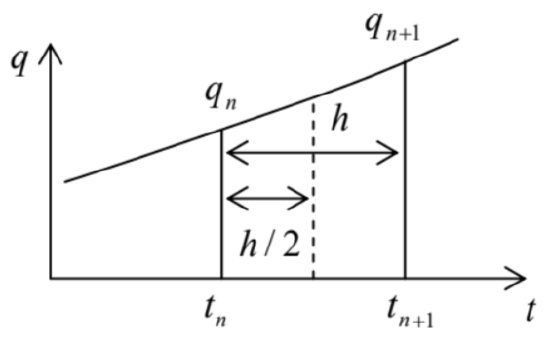 Figure 5.11. The basic notions used at numerical integration of ordinary differential equations.
In the simplest approach (called the Euler method), \(q_{n+1}\) is found using the following formula: \[\begin{aligned} &q_{n+1}=q_{n}+k, \\ &k \equiv h f\left(t_{n}, q_{n}\right) . \end{aligned}\] This approximation is equivalent to the replacement of the genuine function \(q(t)\), on the segment \(\left[t_{n}\right.\), \(t_{n+1}\) ], with the two first terms of its Taylor expansion in point \(t_{n}\) : \[q\left(t_{n}+h\right) \approx q\left(t_{n}\right)+\dot{q}\left(t_{n}\right) h \equiv q\left(t_{n}\right)+h f\left(t_{n}, q_{n}\right) .\] This approximation has an error proportional to \(h^{2}\). One could argue that making the step \(h\) sufficiently small, the Euler method’s error might be made arbitrarily small, but even with all the number-crunching power of modern computer platforms, the CPU time necessary to reach sufficient accuracy may be too large for large problems. \({ }^{35}\) Besides that, the increase of the number of time steps, which is necessary at \(h \rightarrow 0\) at a fixed total time interval, increases the total rounding errors and eventually may cause an increase, rather than the reduction of the overall error of the computed result.
A more efficient way is to modify Eq. (96) to include the terms of the second order in \(h\). There are several ways to do this, for example using the \(2^{\text {nd }}\)-order Runge-Kutta method: \[\begin{aligned} &q_{n+1}=q_{n}+k_{2}, \\ &k_{2} \equiv h f\left(t_{n}+\frac{h}{2}, q_{n}+\frac{k_{1}}{2}\right), \quad k_{1} \equiv h f\left(t_{n}, q_{n}\right) . \end{aligned}\] One can readily check that this method gives the exact result if the function \(q(t)\) is a quadratic polynomial, and hence in the general case its errors are of the order of \(h^{3}\). We see that the main idea here is to first break the segment \(\left[t_{n}, t_{n+1}\right]\) in half (see Figure 11), evaluate the right-hand side of the differential equation (95) at the point intermediate (in both \(t\) and \(q\) ) between the points number \(n\) and \((n+1)\), and then use this information to predict \(q_{n+1}\).
The advantage of the Runge-Kutta approach over other second-order methods is that it may be readily extended to the \(4^{\text {th }}\) order, without an additional breakup of the interval \(\left[t_{n}, t_{n+1}\right] .:\) \[\begin{aligned} &q_{n+1}=q_{n}+\frac{1}{6}\left(k_{1}+2 k_{2}+2 k_{3}+k_{4}\right), \\ &k_{4} \equiv h f\left(t_{n}+h, q_{n}+k_{3}\right), k_{3} \equiv h f\left(t_{n}+\frac{h}{2}, q_{n}+\frac{k_{2}}{2}\right), k_{2} \equiv h f\left(t_{n}+\frac{h}{2}, q_{n}+\frac{k_{1}}{2}\right), k_{1} \equiv h f\left(t_{n}, q_{n}\right) . \end{aligned}\] This method has a much lower error, \(O\left(h^{5}\right)\), without being not too cumbersome. These features have made the \(4^{\text {th }}\)-order Runge-Kutta the default method in most numerical libraries. Its extension to higher orders is possible, but requires more complex formulas, and is justified only for some special cases, e.g., very abrupt functions \(q(t) .{ }^{36}\) The most frequent enhancement of the method is an automatic adjustment of the step \(h\) to reach the pre-specified accuracy, but not make more calculations than necessary.
Figure 12 shows a typical example of an application of that method to the very simple problem of a damped linear oscillator, for two values of fixed time step \(h\) (expressed in terms of the number \(N\) of such steps per oscillation period). The black straight lines connect the adjacent points obtained by the \(4^{\text {th }}\)-order Runge-Kutta method, while the points connected with the green straight lines represent the exact analytical solution (22). The plots show that a-few-percent errors start to appear only at as few as \(\sim 10\) time steps per period, so that the method is indeed very efficient.
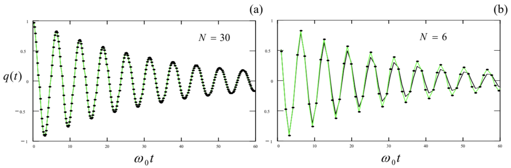
Figure 5.12. Results of the Runge-Kutta solution of Eq. (6) (with \(\delta / \omega_{0}=0.03\) ) for: (a) 30 and (b) 6 points per oscillation period. The results are shown by points; the black and green lines are only the guides for the eye.
Let me hope that the discussion in the next section will make the conveniences and the handicaps of the numerical approach to problems of nonlinear dynamics very clear.
\({ }^{35}\) In addition, the Euler method is not time-reversible - the handicap that may be essential for the integration of Hamiltonian systems described by systems of second-order differential equations. However, this drawback may be partly overcome by the so-called leapfrogging - the overlap of time steps \(h\) for a generalized coordinate and the corresponding generalized velocity.
\({ }^{36}\) The most popular approaches in such cases are the Richardson extrapolation, the Bulirsch-Stoer algorithm, and a set of so-called prediction-correction techniques, e.g. the Adams-Bashforth-Moulton method - see the literature recommended in MA Sec. 16(iii).