6.3: 1D Waves

The second case when the general results of the last section may be simplified are coupled systems with a considerable degree of symmetry. Perhaps the most important of them are uniform systems that may sustain traveling and standing waves. Figure 4a shows a simple example of such a system - a long uniform chain of particles, of mass \(m\), connected with light, elastic springs, prestretched with the tension force \(\mathscr{T}\) to have equal lengths \(d\). (To some extent, this is a generalization of the two-particle system considered in Sec. \(1-\) cf. Figure 1.)

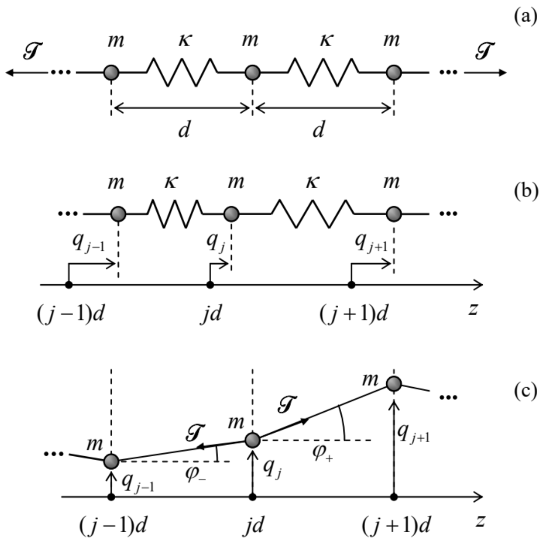Fig. 6.4. (a) A uniform 1D chain of elastically coupled particles, and their small (b) longitudinal and (c) transverse displacements (much exaggerated for clarity).

The spring’s pre-stretch does not affect small longitudinal oscillations \(q_{j}\) of the particles about their equilibrium positions \(z_{j}=j d\) (where the integer \(j\) numbers the particles sequentially) \(-\) see Figure \(4 \mathrm{~b} .{ }^{5}\) Indeed, in the \(2^{\text {nd }}\) Newton law for such a longitudinal motion of the \(j^{\text {th }}\) particle, the forces \(\mathscr{T}\) and \(-\mathscr{T}\) exerted by the springs on the right and the left of it, cancel. However, elastic additions, \(\kappa \Delta q\), to these forces are generally different: \[m \ddot{q}_{j}=\kappa\left(q_{j+1}-q_{j}\right)-\kappa\left(q_{j}-q_{j-1}\right) .\] On the contrary, for transverse oscillations within one plane (Figure 4c), the net transverse component of the pre-stretch force exerted on the \(j^{\text {th }}\) particle, \(\mathscr{T}_{\mathrm{t}}=\mathscr{T}\left(\sin \varphi_{+}-\sin \varphi_{-}\right)\), where \(\varphi_{\pm}\)are the force direction angles, does not vanish. As a result, direct contributions into this force from small transverse oscillations, with \(\left|q_{j}\right|<<d, \mathscr{T} \kappa\), are negligible. Also, due to the first of these strong conditions, the angles \(\varphi_{\pm}\)are small, and hence may be approximated, respectively, as \(\varphi_{+} \approx\left(q_{j+1}-q_{j}\right) / d\) and \(\varphi_{-} \approx\left(q_{j}-q_{j-1}\right) / d\). Plugging these expressions into a similar approximation, \(\mathscr{T}_{\mathrm{t}} \approx \mathscr{T} \varphi_{+}-\varphi_{-}\)) for the transverse force, we see that it may be expressed as \(\mathscr{T}\left(q_{j+1}-q_{j}\right) / d-\mathscr{T}\left(q_{j}-q_{j-1}\right) / d\), i.e. is absolutely similar to that in the longitudinal case, just with the replacement \(\kappa \rightarrow \mathscr{T} / d\). As a result, we may write the equation of motion of the \(j^{\text {th }}\) particle for these two cases in the same form: \[m \ddot{q}_{j}=\kappa_{\mathrm{ef}}\left(q_{j+1}-q_{j}\right)-\kappa_{\mathrm{ef}}\left(q_{j}-q_{j-1}\right),\] where \(\kappa_{\text {ef }}\) is the "effective spring constant", equal to \(\kappa\) for the longitudinal oscillations, and to \(\mathscr{T} / d\) for the transverse oscillations. \({ }^{6}\)Apart from the (formally) infinite size of the system, Eq. (24) is just a particular case of Eq. (17), and thus its particular solution may be looked for in the form (18), where in the light of our previous experience, we may immediately take \(\lambda^{2} \equiv-\omega^{2}\). With this substitution, Eq. (24) gives the following simple form of the general system of equations (17) for the distribution coefficients \(c_{j}\) : \[\left(-m \omega^{2}+2 \kappa_{\mathrm{ef}}\right) c_{j}-\kappa_{\mathrm{ef}} c_{j+1}-\kappa_{\mathrm{ef}} c_{j-1}=0 .\] Now comes the most important conceptual step toward the wave theory. The translational symmetry of Eq. (25), i.e. its invariance to the replacement \(j \rightarrow j+1\), allows it to have particular solutions of the following form: \[c_{j}=a e^{i \alpha j}\] where the coefficient \(\alpha\) may depend on \(\omega\) (and system’s parameters), but not on the particle number \(j\). Indeed, plugging Eq. (26) into Eq. (25) and canceling the common factor \(e^{i \alpha j}\), we see that it is indeed identically satisfied, provided that \(\alpha\) obeys the following algebraic equation: \[\left(-m \omega^{2}+2 \kappa_{\mathrm{ef}}\right)-\kappa_{\mathrm{ef}} e^{+i \alpha}-\kappa_{\mathrm{ef}} e^{-i \alpha}=0 .\] The physical sense of the solution (26) becomes clear if we use it and Eq. (18) with \(\lambda=\mp i \omega\), to write \[q_{j}(t)=\operatorname{Re}\left[a \exp \left\{i\left(k z_{j} \mp \omega t\right)\right\}\right]=\operatorname{Re}\left[a \exp \left\{i k\left(z_{j} \mp v_{\mathrm{ph}} t\right)\right\}\right]\] where the wave number \(k\) is defined as \(k \equiv \alpha / d\). Eq. (28) describes a sinusoidal \({ }^{7}\) traveling wave of particle displacements, which propagates, depending on the sign before \(v_{\mathrm{ph}}\), to the right or the left along the particle chain, with the so-called phase velocity \[v_{\mathrm{ph}} \equiv \frac{\omega}{k} .\] Perhaps the most important characteristic of a wave system is the so-called dispersion relation, i.e. the relation between the wave’s frequency \(\omega\) and its wave number \(k-\) one may say, between the temporal and spatial frequencies of the wave. For our current system, this relation is given by Eq. (27) with \(\alpha \equiv k d\). Taking into account that \(\left(2-e^{+i \alpha}-e^{-i \alpha}\right) \equiv 2(1-\cos \alpha) \equiv 4 \sin ^{2}(\alpha / 2)\), the dispersion relation may be rewritten in a simpler form: \[\omega=\pm \omega_{\max } \sin \frac{\alpha}{2} \equiv \pm \omega_{\max } \sin \frac{k d}{2}, \quad \text { where } \omega_{\max } \equiv 2\left(\frac{\kappa_{\mathrm{ef}}}{m}\right)^{1 / 2}\] This result, sketched in Figure 5, is rather remarkable in several aspects. I will discuss them in detail, because most of these features are typical for waves of any type (including even the "de Broglie waves", i.e. wavefunctions, in quantum mechanics), propagating in periodic structures.

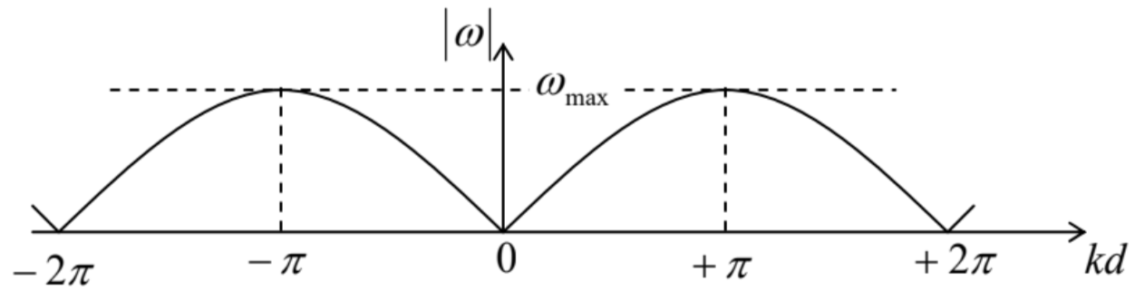
Fig. 6.5. The dispersion relation (30).

First, at low frequencies, \(\omega<<\omega_{\max }\), the dispersion relation (31) is linear: \[\omega=\pm v k, \quad \text { where } v \equiv\left|\frac{d \omega}{d k}\right|_{k=0}=\frac{\omega_{\max } d}{2}=\left(\frac{\kappa_{\mathrm{ef}}}{m}\right)^{1 / 2} d .\] Plugging Eq. (31) into Eq. (29), we see that the constant \(v\) plays, in the low-frequency limit, the role of the same phase velocity for waves of any frequency. Due to its importance, this acoustic wave limit will with the subject of the special next section.

Second, when the wave frequency is comparable with \(\omega_{\max }\), the dispersion relation is not linear, and the system is dispersive. This means that as a wave, whose Fourier spectrum has several essential components with frequencies of the order of \(\omega_{\max }\), travels along the structure, its waveform (which may be defined as the shape of the line connecting all points \(q_{j}(z)\), at the same time) changes. \({ }^{9}\) This effect may be analyzed by representing the general solution of Eq. (24) as the sum (more generally, an integral) of the components (28) with different complex amplitudes \(a\) : \[q_{j}(t)=\operatorname{Re} \int_{-\infty}^{+\infty} a_{k} \exp \left\{i\left[k z_{j}-\omega(k) t\right]\right\} d k .\] This notation emphasizes the dependence of the component wave amplitudes \(a_{k}\) and frequencies \(\omega\) on the wave number \(k\). While the latter dependence is given by the dispersion relation (in our current case by Eq. (30)), the function \(a_{k}\) is determined by the initial conditions. For applications, the case when \(a_{k}\) is substantially different from zero only in a narrow interval, of a width \(\Delta k<<k_{0}\) around some central value \(k_{0}\), is of special importance. The Fourier transform reciprocal to Eq. (32) shows that this is true, in particular, for the so-called wave packet - a sinusoidal wave modulated by a spatial envelope function of a large width \(\Delta z \sim 1 / \Delta k>>1 / k_{0}-\) see, e.g., Figure 6 .

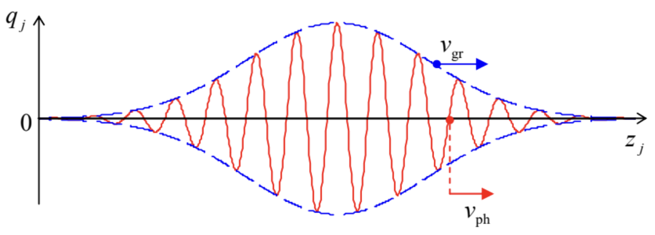Figure 6.6. The phase and group velocities of a wave packet.

Using the strong inequality \(\Delta k<<k_{0}\), the wave packet’s propagation may be analyzed by expending the dispersion relation \(\omega(k)\) into the Taylor series at point \(k_{0}\), and, in the first approximation in \(\Delta k / k_{0}\), restricting the expansion to its first two terms: \[\omega(k) \approx \omega_{0}+\left.\frac{d \omega}{d k}\right|_{k=k_{0}} \tilde{k}, \quad \text { where } \omega_{0} \equiv \omega\left(k_{0}\right), \text { and } \widetilde{k} \equiv k-k_{0} .\] In this approximation, Eq. (32) yields \[\begin{aligned} q_{j}(t) & \approx \operatorname{Re} \int_{-\infty}^{+\infty} a_{k} \exp \left\{i\left[\left(k_{0}+\tilde{k}\right) z_{j}-\left(\omega_{0}+\frac{d \omega}{d k} \mid k=k_{0} \tilde{k}\right) t\right]\right\} d k \\ & \equiv \operatorname{Re}\left[\exp \left\{i\left(k_{0} z_{j}-\omega_{0} t\right)\right\} \int_{-\infty}^{+\infty} a_{k} \exp \left\{i \widetilde{k}\left(z_{j}-\left.\frac{d \omega}{d k}\right|_{k=k_{0}} t\right)\right\} d k\right] . \end{aligned}\] Comparing the last expression with the initial form of the wave packet, \[q_{j}(0)=\operatorname{Re} \int_{-\infty}^{+\infty} a_{k} e^{i k z_{j}} d k \equiv \operatorname{Re}\left[\exp \left\{i k_{0} z_{j}\right\} \int_{-\infty}^{+\infty} a_{k} \exp \left\{\tilde{k} z_{j}\right\} d k\right],\] and taking into account that the phase factors before the integrals in the last forms of Eqs. (34) and (35) do not affect its envelope, we see that in this approximation the envelope sustains its initial form and propagates along the system with the so-called group velocity \[\left.v_{\mathrm{gr}} \equiv \frac{d \omega}{d k}\right|_{k=k_{0}} .\] Except for the acoustic wave limit (31), this velocity, which characterizes the propagation of waveform’s envelope, is different from the phase velocity (29), which describes the propagation of the "carrier" sinusoidal wave, e.g., the position of one of its zeros - see the red and blue arrows in Figure 6 . (Taking into account the next term in the Taylor expansion of the function \(\omega(q)\), proportional to \(d^{2} \omega / d q^{2}\), we would find that the dispersion leads to a gradual change of the envelope’s form. Such changes play an important role in quantum mechanics, so that they are discussed in detail in the QM part of these lecture notes.) Next, for our particular dispersion relation (30), the difference between \(v_{\mathrm{ph}}\) and \(v_{\mathrm{gr}}\) increases as \(\omega\) approaches \(\omega_{\max }\), with the group velocity (36) tending to zero, while the phase velocity staying almost constant. The physics of such a maximum frequency available for the wave propagation may be readily understood by noticing that according to Eq. (30), at \(\omega=\omega_{\max }\), the wave number \(k\) equals \(n \pi / d\), where \(n\) is an odd integer, and hence the phase shift \(\alpha \equiv k d\) is an odd multiple of \(\pi\). Plugging this value into Eq. (28), we see that at \(\omega=\omega_{\max }\), the oscillations of two adjacent particles are in anti-phase, for example: \[q_{0}(t)=\operatorname{Re}[a \exp \{-i \omega t\}], \quad q_{1}(t)=\operatorname{Re}[a \exp \{i \pi-i \omega t\}]=-q_{0}(t) .\] It is clear, especially from Figure \(4 \mathrm{~b}\) for longitudinal oscillations, that at such a phase shift, all the springs are maximally stretched/compressed (just as in the hard mode of the two coupled oscillators analyzed in Sec. 1), so that it is natural that this mode has the highest possible frequency.

This fact invites a natural question: what happens with the system if it is agitated at a frequency \(\omega>\omega_{\max }\), say by an external force applied at its boundary? Reviewing the calculations that have led to the dispersion relation (30), we see that they are all valid not only for real but also any complex values of \(k\). In particular, at \(\omega>\omega_{\max }\) it gives \[k=\frac{(2 n-1) \pi}{d} \pm \frac{i}{\Lambda}, \quad \text { where } n=1,2,3, \ldots, \quad \Lambda \equiv \frac{d}{2 \cosh ^{-1}\left(\omega / \omega_{\max }\right)} .\] Plugging this relation into Eq. (28), we see that the wave’s amplitude becomes an exponential function of the particle’s position: \[\left|q_{j}\right|=|a| e^{\pm j \operatorname{Im} k d} \propto \exp \left\{\pm z_{j} / \Lambda\right\} .\] Physically this means that penetrating into the structure, the wave decays exponentially (from the excitation point), dropping by a factor of \(e \approx 3\) at the so-called penetration depth \(\Lambda\). (According to Eq. (38), at \(\omega \sim \omega_{\max }\) this depth is of the order of the distance \(d\) between the adjacent particles, and decreases but rather slowly as the frequency is increased beyond \(\omega_{\max }\).) Such a limited penetration is a very common property of waves, including the electromagnetic waves penetrating into various plasmas and superconductors, and the quantum-mechanical de Broglie waves penetrating into classically-forbidden regions of space. Note that this effect of "wave expulsion" from a medium does not require any energy dissipation.

Finally, one more fascinating feature of the dispersion relation (30) is its periodicity: if the relation is satisfied by some wave number \(k_{0}(\omega)\), it is also satisfied at any \(k_{n}(\omega)=k_{0}(\omega)+2 \pi n / d\), where \(n\) is an integer. This property is independent of the particular dynamics of the system and is a common property of all systems that are \(d\)-periodic in the usual ("direct") space. It has especially important implications for the quantum de Broglie waves in periodic systems - for example, crystals - leading, in particular, to the famous band/gap structure of their energy spectrum. \({ }^{10}\)

---

\({ }^{5}\) Note the need a clear distinction between the equilibrium position \(z_{j}\) of the \(j^{\text {th }}\) point and its deviation from it, \(q_{j}\). Such distinction has to be sustained in the continuous limit (see below), where it is frequently called the Eulerian description - named after L. Euler, even though it was introduced to mechanics by J. d’Alembert. In this course, the distinction is emphasized by using different letters - respectively, \(z\) and \(q\). (In the 3D case, \(\mathbf{r}\) and \(\mathbf{q}\).)

\({ }^{6}\) The re-derivation of Eq. (24) from the Lagrangian formalism, with the simultaneous strict proof that the small oscillations in the longitudinal direction and the two mutually perpendicular transverse directions are all independent of each other, is a very good exercise, left for the reader.

\({ }^{7}\) In optics and quantum mechanics, such waves are usually called monochromatic; I will not use this term until the corresponding parts (EM and QM) of my series.

\({ }^{8}\) This term is purely historical. Though the usual sound waves in air belong to this class, the waves we are discussing may have frequencies both well below and well above the human ear’s sensitivity range.

\({ }^{9}\) The waveform deformation due to dispersion (which we are considering now) should be clearly distinguished from its possible change due to attenuation, i.e. energy loss - which is not taken into account is our current energy-conserving model - cf. Sec. 6 below.

\({ }^{10}\) For more detail see, e.g., QM Sec. \(2.5\).