6.2: N Coupled Oscillators

The calculations of the previous section may be readily generalized to the case of an arbitrary number (say, \(N\) ) coupled harmonic oscillators, with an arbitrary type of coupling. It is evident that in this case Eq. (4) should be replaced with \[L=\sum_{j=1}^{N} L_{j}+\sum_{j, j^{\prime}=1}^{N} L_{j j^{\prime}}\] Moreover, we can generalize the above expression for the mixed terms \(L_{j j}\), taking into account their possible dependence not only on the generalized coordinates but also on the generalized velocities, in a bilinear form similar to Eq. (4). The resulting Lagrangian may be represented in a compact form, \[L=\sum_{j, j^{\prime}=1}^{N}\left(\frac{m_{i j^{\prime}}}{2} \dot{q}_{j} \dot{q}_{j^{\prime}}-\frac{\kappa_{i j^{\prime}}}{2} q_{j} q_{j^{\prime}}\right),\] where the off-diagonal terms are index-symmetric: \(m_{j j^{\prime}}=m_{j^{\prime} j}, \kappa_{j j^{\prime}}=\kappa_{j j}\), and the factors \(1 / 2\) compensate the double counting of each term with \(j \neq j\) ’, taking place at the summation over two independently running indices. One may argue that Eq. (16) is quite general if we still want to keep the equations of motion linear - as they always are if the oscillations are small enough.

Plugging Eq. (16) into the general form (2.19) of the Lagrange equation, we get \(N\) equations of motion of the system, one for each value of the index \(j^{\prime}=1,2, \ldots, N:\) \[\sum_{j=1}^{N}\left(m_{i j j} \ddot{q}_{j}+\kappa_{j j^{\prime}} q_{j}\right)=0 .\] Just as in the previous section, let us look for a particular solution to this system in the form \[q_{j}=c_{j} e^{\lambda t} .\] As a result, we are getting a system of \(N\) linear, homogeneous algebraic equations, \[\sum_{j=1}^{N}\left(m_{i j^{\prime}} \lambda^{2}+\kappa_{j j^{\prime}}\right) c_{j}=0,\] for the set of \(N\) distribution coefficients \(c_{j}\). The condition that this system is self-consistent is that the determinant of its matrix equals zero: \[\operatorname{Det}\left(m_{i j^{\prime}} \lambda^{2}+\kappa_{i j^{\prime}}\right)=0 .\] This characteristic equation is an algebraic equation of degree \(N\) for \(\lambda^{2}\), and so has \(N\) roots \(\left(\lambda^{2}\right)_{n}\). For any Hamiltonian system with stable equilibrium, the matrices \(m_{i j}\) ’ and \(\kappa_{i j}\) ’ ensure that all these roots are real and negative. As a result, the general solution to Eq. (17) is the sum of \(2 N\) terms proportional to exp \(\left\{\pm i \omega_{n} t\right\}, n=1,2, \ldots, N\), where all \(N\) eigenfrequencies \(\omega_{n}\) are real.

Plugging each of these \(2 N\) values of \(\lambda=\pm i \omega_{n}\) back into a particular set of linear equations (17), one can find the corresponding set of distribution coefficients \(c_{j \pm}\). Generally, the coefficients are complex, but to keep \(q_{j}(t)\) real, the coefficients \(c_{j+}\) corresponding to \(\lambda=+i \omega_{n}\), and \(c_{j}\) - corresponding to \(\lambda\) \(=-i \omega_{n}\) have to be complex-conjugate of each other. Since the sets of the distribution coefficients may be different for each \(\lambda_{n}\), they should be marked with two indices, \(j\) and \(n\). Thus, at general initial conditions, the time evolution of the \(j^{\text {th }}\) coordinate may be represented as \[q_{j}=\frac{1}{2} \sum_{n=1}^{N}\left(c_{j n} \exp \left\{+i \omega_{n} t\right\}+c_{j n}^{*} \exp \left\{-i \omega_{n} t\right\}\right) \equiv \operatorname{Re} \sum_{n=1}^{N} c_{j n} \exp \left\{i \omega_{n} t\right\}\] This formula shows very clearly again the physical sense of the distribution coefficients \(c_{j n}\) : a set of these coefficients, with different values of index \(j\) but the same \(n\), gives the complex amplitudes of oscillations of the coordinates for the special initial conditions that ensure purely sinusoidal motion of all the system, with frequency \(\omega_{n}\).

The calculation of the eigenfrequencies and distribution coefficients of a particular coupled system with many degrees of freedom from Eqs. (19)-(20) is a task that frequently may be only done numerically. \({ }^{4}\) Let us discuss just two particular but very important cases. First, let all the coupling coefficients be small in the following sense: \(\left|m_{j j^{\prime}}\right|<<m_{j} \equiv m_{j j}\) and \(\left|\kappa_{i j^{\prime}}\right|<<\kappa_{j} \equiv \kappa_{j j}\), for all \(j \neq j\), and all partial frequencies \(\Omega_{j} \equiv\left(\kappa_{j} / m_{j}\right)^{1 / 2}\) be not too close to each other:

\[\ \frac{\left|\Omega_{j}^{2}-\Omega_{j^{\prime}}^{2}\right|}{\Omega_{j}^{2}}>>\frac{\left|\kappa_{j j^{\prime}}\right|}{\kappa_{j}}, \frac{\left|m_{j j^{\prime}}\right|}{m_{j}}, \quad \text { for all } j \neq j^{\prime}.\]

(Such situation frequently happens if parameters of the system are "random" in the sense that they do not follow any special, simple rule - for example, resulting from some simple symmetry of the system.) Results of the previous section imply that in this case, the coupling does not produce a noticeable change of oscillation frequencies: \(\left\{\omega_{n}\right\} \approx\left\{\Omega_{j}\right\}\). In this situation, oscillations at each eigenfrequency are heavily concentrated in one degree of freedom, i.e. in each set of the distribution coefficients \(c_{j n}\) (for a given \(n\) ), one coefficient’s magnitude is much larger than all others.

Now let the conditions (22) be valid for all but one pair of partial frequencies, say \(\Omega_{1}\) and \(\Omega_{2}\), while these two frequencies are so close that coupling of the corresponding partial oscillators becomes essential. In this case, the approximation \(\left\{\omega_{n}\right\} \approx\left\{\Omega_{j}\right\}\) is still valid for all other degrees of freedom, and the corresponding terms may be neglected in Eqs. (19) for \(j=1\) and 2 . As a result, we return to Eqs. (7) (perhaps generalized for velocity coupling) and hence to the anticrossing diagram (Figure 2) discussed in the previous section. As a result, an extended change of only one partial frequency (say, \(\Omega_{1}\) ) of a weakly coupled system produces a sequence of eigenfrequency anticrossings - see Figure 3 .

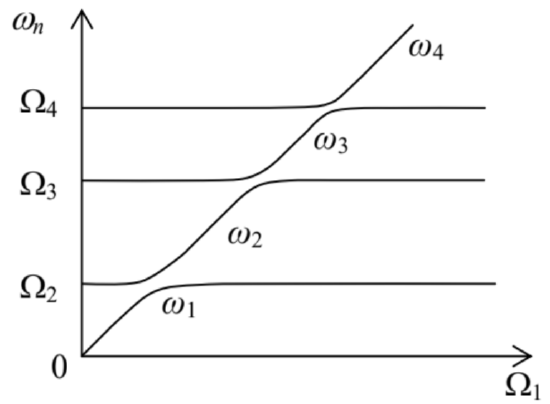
Figure 6.3. The level anticrossing in a system of \(N\) weakly coupled oscillators - schematically.

---

\({ }^{4}\) Fortunately, very effective algorithms have been developed for this matrix diagonalization task - see, e.g., references in MA Sec. 16(iii)-(iv). For example, the popular MATLAB software package was initially created exactly for this purpose. ("MAT" in its name stands for "matrix" rather than "mathematics".)