
6.4: Acoustic Waves


- Last updated
- Jan 27, 2022
- Save as PDF

( \newcommand{\kernel}{\mathrm{null}\,}\)
Now let us return to the limit of low-frequency, dispersion-free acoustic waves, with |ω|<<ω0, propagating with the frequency-independent velocity (31). Such waves are the general property of any elastic continuous medium and obey a simple (and very important) partial differential equation. To derive it, let us note that in the acoustic wave limit, |kd|<<1,11 the phase shift α≡kd is very close to 2πn. This means that the differences qj+1(t)−qj(t) and qj(t)−qj−1(t), participating in Eq. (25), are relatively small and may be approximated with ∂q/∂j≡∂q/∂(z/d)≡d(∂q/∂z), with the derivatives taken at middle points between the particles: respectively, z+≡(zj+1−zj)/2 and z−≡(zj−zj−1)/2. Let us now consider z as a continuous argument, and introduce the particle displacement q(z,t)− a continuous function of space and time, satisfying the requirement q(zj,t)=qj(t). In this notation, in the limit kd →0, the sum of the last two terms of Eq. (24) becomes −κd[∂q/∂z(z+)−∂q/∂z(z−)], and hence may be approximated as −κd2(∂2q/∂z2), with the second derivative taken at point (z+−z−)/2≡zj, i.e. exactly at the same point as the time derivative. As the result, the whole set of ordinary differential equations (24), for different j, is reduced to just one partial differential equation m∂2q∂t2−κef d2∂2q∂z2=0. Using Eq. (31), we may rewrite this 1D wave equation in a more general form (1v2∂2∂t2−∂2∂z2)q(z,t)=0 The most important property of the wave equation (40), which may be verified by an elementary substitution, is that it is satisfied by either of two traveling wave solutions (or their linear superposition): q+(z,t)=f+(t−z/v),q−(z,t)=f−(t+z/v), where f±are any smooth functions of one argument. The physical sense of these solutions may be revealed by noticing that the displacements q±do not change at the addition of an arbitrary change Δt to their time argument, provided that it is accompanied by an addition of the proportional addition of ∓vΔt to their space argument. This means that with time, the waveforms just move (respectively, to the left or the right), with the constant speed v, retaining their form - see Figure 7. 12
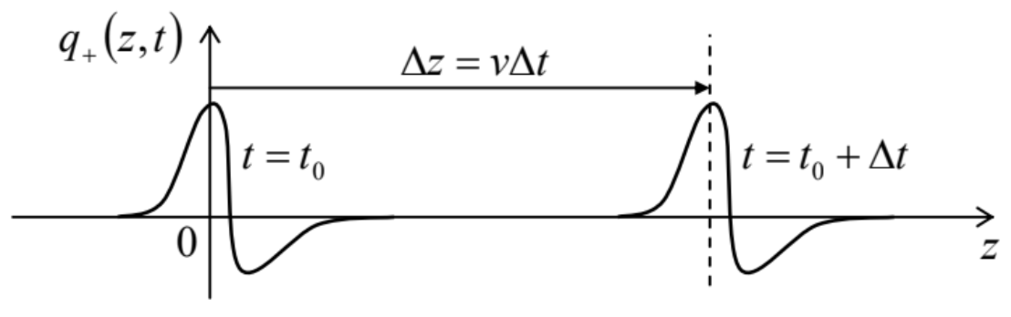 Fig. 6.7. Propagation of a traveling wave in a dispersion-free 1D system.
Returning to the simple model shown in Figure 4, let me emphasize that the acoustic-wave velocity v is different for the waves of two types: for the longitudinal waves (with κef=κ, see Figure 4b), v=vl≡(κm)1/2d, while for the transverse waves (with κef=T/d, see Figure 4c): v=vt=(Tmd)1/2d≡(Jdm)1/2≡(Tμ)1/2 where the constant μ≡m/d has a simple physical sense of the particle chain’s mass per unit length. Evidently, these velocities, in the same system, may be rather different.The wave equation (40), with its only parameter v, may conceal the fact that any wavesupporting system is characterized by one more key parameter. In our current model (Figure 4), this parameter may be revealed by calculating the forces F±(z,t) accompanying any of the traveling waves (41) of particle displacements. For example, in the acoustic wave limit kd→0 we are considering now, the force exerted by the jth particle on its right neighbor may be approximated as F(zj,t)≡κef[qj(t)−qj+1(t)]≈−κef∂q∂z|z=zjd, where, as was discussed above, κef equals κ for the longitudinal waves, and to T/d for the transverse waves. But for the traveling waves (41), the partial derivatives ∂q±/∂z are equal to ∓(df±/dt)/v, so that the corresponding forces are equal to F±=∓κefdvdf±dt, i.e. are proportional to the particle’s velocities u=∂q/∂t in these waves, 13u±=df±/dt, for the same z and t. This means that the ratio F±(z,t)u±(z,t)=−κefd∂q±/∂z∂q±/∂t=−κefd(∓df±/dt)/vdf±/dt≡±κefdv, depends only on the wave propagation direction, but is independent of z and t, and also of the propagating waveform. Its magnitude, Z≡|F±(z,t)u±(z,t)|=κefdv=(κefm)1/2, characterizing the dynamic "stiffness" of the system for the propagating waves, is called the wave impedance. 14 Note that the impedance is determined by the product of the system’s generic parameters κef and m, while the wave velocity (31) is proportional to their ratio, so that these two parameters are completely independent, and both are important. According to Eq. (47), the wave impedance, just as the wave velocity, is also different for the longitudinal and transverse waves:
Zl=κdνl≡(κm)1/2,Zt=Tνt≡(Tμ)1/2.
(Note that the first of these expressions for Z coincides with the one used for a single oscillator in Sec. 5.6. In that case, Z may be also recast in a form similar to Eq. (46), namely, as the ratio of the force and velocity amplitudes at free oscillations.)
One of the wave impedance’s key functions is to scale the power carried by a traveling wave: P±≡F±(z,t)u±(z,t)=−κefd∂q±∂z∂q±∂t=±κefdv(df±dt)2≡±Z(df±dt)2. Two remarks about this important result. First, the sign of P depends only on the direction of the wave propagation, but not on the waveform. Second, the instant value of the power does not change if we move with the wave in question, i.e. measure P at points with z±vt= const. This is natural because in the Hamiltonian system we are considering, the wave energy is conserved. Hence, the wave impedance Z characterizes the energy transfer along the system rather than its dissipation.
Another important function of the wave impedance notion becomes clear when we consider waves in nonuniform systems. Indeed, our previous analysis assumed that the 1D system supporting the waves (Figure 4) is exactly periodic, i.e. macroscopically uniform, and extends all the way from −∞ to +∞. Now let us examine what happens when this is not true. The simplest, and very important example of such nonuniform systems is a sharp interface, i.e. a point (say, z=0 ) at which system parameters experience a jump while remaining constant on each side of the interface − see Figure 8.
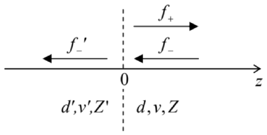 Figure 6.8. Partial reflection of a wave from a sharp interface.
In this case, the wave equation (40) and its partial solutions (41) are is still valid for z⟨0 and z⟩ 0 - in the former case, with primed parameters. However, the jump of parameters at the interface leads to a partial reflection of the incident wave from the interface, so that at least on the side of the incidence (in the case shown in Figure 8, for z≥0 ), we need to use two such terms, one describing the incident wave and another one, the reflected wave: q(z,t)={f′−(t+z/v′), for z≤0,f−(t+z/v)+f+(t−z/v), for z≥0. To find the relations between the functions f−,f+, and f−’ (of which the first one, describing the incident wave, may be considered known), we may use two boundary conditions at z=0. First, the displacement q0(t) of the particle at the interface has to be the same whether it is considered a part of the left or right sub-system, and it participates in Eqs. (50) for both z≤0 and z≥0. This gives us the first boundary condition: f′−(t)=f−(t)+f+(t). On the other hand, the forces exerted on the interface from the left and the right should also have equal magnitude, because the interface may be considered as an object with a vanishing mass, and any nonzero net force would give it an infinite (and hence unphysical) acceleration. Together with Eqs. (45) and (47), this gives us the second boundary condition: Z′df′−(t)dt=Z[df−(t)dt−df+(t)dt]. Integrating both parts of this equation over time, and neglecting the integration constant (which describes a common displacement of all particles rather than their oscillations), we get Z′f′−(t)=Z[f−(t)−f+(t)]. Now solving the system of two linear equations (51) and (53) for f+(t) and f′+(t), we see that both these functions are proportional to the incident waveform: f+(t)=Rf−(t),f′−(t)=τf−(t), with the following reflection (R) and transmission (T) coefficients: R=Z−Z′Z+Z′,τ=2ZZ+Z′. Later in this series, we will see that with the appropriate re-definition of the impedance, these relations are also valid for waves of other physical nature (including the de Broglie waves in quantum mechanics) propagating in 1D continuous structures, and also in continua of higher dimensions, at the normal wave incidence upon the interface. 15 Note that the coefficients R and T give the ratios of wave amplitudes, rather than their powers. Combining Eqs. (49) and (55), we get the following relations for the powers - either at the interface or at the corresponding points of the reflected and transmitted waves: P+=(Z−Z′Z+Z′)2P−,P′−=4ZZ′(Z+Z′)2P−. Note that P−+P+=P′−, , again reflecting the wave energy conservation.
Perhaps the most important corollary of Eqs. (55)-(56) is that the reflected wave completely vanishes, i.e. the incident wave is completely transmitted through the interface (P′+=P+), if the socalled impedance matching condition Z′=Z is satisfied, even if the wave velocities v(32) are different on the left and the right sides of it. On the contrary, the equality of the acoustic velocities in the two continua does not guarantee the full transmission of their interface. Again, this is a very general result.
Finally, let us note that for the important particular case of a sinusoidal incident wave: 16 f−(t)=Re[ae−iωt], so that f+(t)=Re[Rae−iωt], where a is its complex amplitude, the total wave (50) on the right of the interface is q(z,t)=Re[ae−iω(t+z/v)+Rae−iω(t−z/v)]≡Re[a(e−ikz+Re+ikz)e−iωt], for z≥0 while according to Eq. (45), the corresponding force distribution is F(z,t)=F−(z,t)+F+(z,t)=−Z∂f−(t−z/v)∂t+Z∂f−(t−z/v)∂t=Re[iωZa(e−ikz−Re+ikz)e−iωt]. These expressions will be used in the next section.
11 Strictly speaking, per the discussion at the end of the previous section, in this reasoning k means the distance of the wave number from the closest point 2πn/d− see Figure 5 again.
12 From the point of view of Eq. (40), the only requirement to the "smoothness" of the functions f±is to be doubly differentiable. However, we should not forget that in our case the wave equation is only an approximation of the discrete Eq. (24), so that according to Eq. (30), the traveling waveform conservation is limited by the acoustic wave limit condition ω<<ωmax, which should be fulfilled for any Fourier component of these functions.
13 Of course, the particle’s velocity u (which proportional to the wave amplitude) should not be confused with the wave’s velocity v (which is independent of this amplitude).
14 This notion is regretfully missing from many physics (but not engineering!) textbooks.
15 See, the corresponding parts of the lecture notes: QM Sec. 2.3 and EM Sec. 7.3.
16 In the acoustic wave limit, when the impedances Z and Z′, and hence the reflection coefficient R, are real, R and Z may be taken from under the Re operators in Eqs. (57)-(59). However, in the current, more general form of these relations they are also valid for the case of arbitrary frequencies, ω∼ωmax, when R and Z may be complex.